The history of mathematics: A brief course (2013)

Part IV. India, China, and Japan 500 BCE-1700 CE

Chapter 23. Later Chinese Algebra and Geometry

We begin our examination of Chinese algebra by taking a brief look at number theory in China. Unlike the Greeks, Chinese mathematicians were not interested in figurate numbers. Still, there was in China an interest in the use of numbers for divination. According to Li and Du (1987, pp. 95–97), the magic square

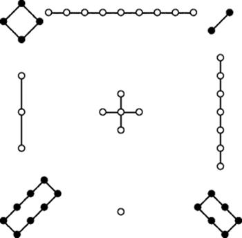
appears in the treatise Shushu Jiyi (Memoir on Some Traditions of the Mathematical Art) by the sixth-century mathematician Zhen Luan. In this figure each row, column, and diagonal totals 15. In the early tenth century, during the Song Dynasty, a connection was made between this magic square and a figure called the Luo-chu-shu (book that came out of the River Lo) found in an appendix to the Book of Changes. The Book of Changes states that a tortoise crawled out of the River Lo and delivered to the Emperor Yu the diagram in Fig. 23.1. Because of this connection, the diagram came to be called the Luo-shu (Luo book). The purely numerical aspects of the magic square are enhanced by representing the even (female, ying) numbers as solid disks and the odd (male, yang) numbers as open circles. Like so much of number theory, the theory of magic squares has continued to attract attention from specialists, despite being devoid of applications. The interest has come from combinatoricists, for whom Latin squares¹ are a topic of continuing research.

Figure 23.1 The Luo-shu.

23.1 Algebra

The development of algebra in China began early and continued for many centuries. The aim was to find numerical approximate solutions to equations, and the Chinese mathematicians were not intimidated by equations of high degree.

23.1.1 Systems of Linear Equations

Systems of linear equations occur in the Jiu Zhang Suan Shu (Mikami, 1913, pp. 18–22; Li and Du, 1987, pp. 46–49). Here is one example of the technique.

There are three kinds [of wheat]. The grains contained in two, three and four bundles, respectively, of these three classes [of wheat], are not sufficient to make a whole measure. If, however, we add to them one bundle of the second, third, and first classes, respectively, then the grains would become one full measure in each case. How many measures of grain does then each one bundle of the different classes contain?

The following counting-board arrangement is given for this problem.

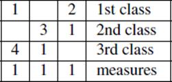
Here the three columns of numbers from right to left represent the three samples of wheat. Thus the right-hand column represents 2 bundles of the first class of wheat, to which one bundle of the second class has been added. The bottom row gives the result in each case: 1 measure of wheat. The word problem might be clearer if the final result is thought of as the result of threshing the raw wheat to produce pure grain. Without seriously distorting the procedure followed by the author, we can write down this counting board as a matrix and solve the resulting system of three equations in three unknowns. The author gives the solution: A bundle of the first type of wheat contains measure, a bundle of the second contains measure, and a bundle of the third contains measure.

23.1.2 Quadratic Equations

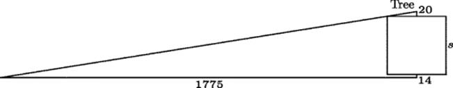
The last chapter of the Jiu Zhang Suan Shu, which involves right triangles, contains problems that lead to linear and quadratic equations. For example (Mikami, 1913, p. 24), there are several problems involving a town enclosed by a square wall with a gate in the center of each side. In some cases the problem asks at what distance (x) from the south gate a tree a given distance east of the east gate will first be visible. The data are the side s of the square and the distance d of the tree from the gate. For that kind of data, the problem is the linear equation 2x/s = s/(2d). When the side of the town (s) is the unknown, a quadratic equation results. In one case, it is asserted that the tree is 20 paces north of the north gate and is just visible to a person who walks 14 paces south of the south gate, then 1775 paces west. This problem proposes the quadratic equation s² + 34s = 71000 to be solved for the unknown side s. (See Fig. 23.2, which is drawn to scale to show how unrealistic the problem really is.) Since the Chinese technique of solving equations numerically is practically independent of degree, we shall not bother to discuss the techniques for solving quadratic equations separately.

Figure 23.2 A quadratic equation problem from the Jiu Zhang Suan Shu.

23.1.3 Cubic Equations

Cubic equations first appear in Chinese mathematics (Li and Du, 1987, p. 100; Mikami, 1913, p. 53) in the seventh-century work Xugu Suanjing (Continuation of Ancient Mathematics) by Wang Xiaotong (ca. 580–ca. 640). This work contains some intricate problems associated with right triangles. For example, compute the length of a leg of a right triangle given that the product of the other leg and the hypotenuse is and the difference between the hypotenuse and the leg is . (Mikami gives as the difference, which is incompatible with the answer given by Wang Xiaotong. I do not know if the mistake is due to Mikami or is in the original.) This problem is easy to state for a general product P and difference D. Wang Xiaotong gives a general description of the result of eliminating the hypotenuse and the other leg that amounts to the equation

In the present case (using the corrected data) the equation is

Wang Xiaotong then gives the root (correctly) as “according to the rule of the cubic root extraction.” Li and Du (1987, pp. 118–119) report that the eleventh-century mathematician Jia Xian developed a method for extracting the cube root that generalizes from the case of the equation x³ = N to the general cubic equation, and even to an equation of arbitrarily high degree, at least in theory, as we shall now see.

23.1.4 A Digression on the Numerical Solution of Equations

The Chinese mathematicians of 800 years ago invented a method of finding numerical approximations of a root of an equation, similar to a method that was rediscovered independently in the nineteenth century in Europe and is commonly called Horner's method, in honor of the British school teacher William Horner (1786–1837).² The first appearance of the method is in the work of the thirteenth-century mathematician Qin Jiushao, who applied it in his 1247 treatise Sushu Jiu Zhang (Arithmetic in Nine Chapters, not to be confused with the Jiu Zhang Suan Shu).

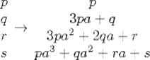
We illustrate with the case of the cubic equation. Suppose in attempting to solve the cubic equation px³ + qx² + rx + s = 0 we have found an initial approximation a for the root. (Typically, this is done by getting the first digit or the integer part of the root.) We then “reduce” the equation by setting x = y + a and rewriting it. What will the coefficients be when the equation is written in terms of y? The answer is immediate; the new equation is

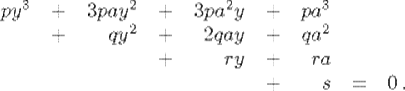
We see that we need to make the following conversion of the coefficients:

Here is a method of making this reduction that is well adapted for use on a counting board.

1. Step 1: By inspection, find a first approximation to a root. (Simply evaluate the polynomial at, say 1, 10, 100, and so on, finding out where it changes sign from negative to positive or vice versa. If it is negative at 10 and positive at 100, for example, then evaluate it at 20, 30, 40, and so on, until you find again where it changes sign. If it is negative at 30 and positive at 40, for example, then you can take 30 as the first approximation.)

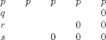
2. Step 2: Lay out a template in the form of a 4 × 5 matrix (for cubic equations), in which (1) all the entries in the top row are the same, namely the leading coefficient, (2) the first column is the coefficients, in order, and (3) the lower right triangle consists of zeros. Thus, we get the matrix

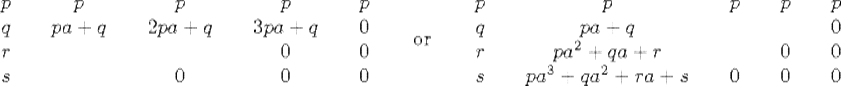
3. Step 3: Fill in the rest of the entries working from left to right and top to bottom (in either order). In each unoccupied place, put the product of the current approximation a and the entry directly above, plus the entry directly to the left. Thus, we could begin by filling in either the second row or the second column:

When we finish, we have the following matrix, and the coefficients are read, in order, off the diagonal running from the top right to the bottom of the second column:

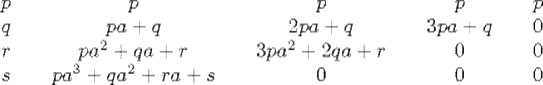
Thus, as we see, the new equation for y is

The zeros used to form the template for the algorithm have a very important use when the solution is being obtained one digit at a time. It is useful to have a solution between 0 and 10 at each stage, and one way to ensure that, after the integer part of the solution (say a) has been obtained, is to multiply the fractional part y by 10. Then one need only seek the integer part of z = 10y. Since z satisfies

and the entries in the matrix will often be integers, one can simply adjoin the zeros to the coefficients when forming the new equation, which necessarily has a solution between 0 and 10.

Wang Xiaotong's reference to the use of cube root extraction for solving his equation seems to suggest that this method was known as early as the seventh century. The earliest recorded instance of it, however, seems to be in the treatise of Qin Jiushao, who illustrated it by solving the quartic equation

The method of solution gives proof that the Chinese did not think in terms of a quadratic formula. If they had, this equation would have been solved for x² using that formula and then x could have been found by taking the square root of any positive root. But Qin Jiushao applied the fourth-degree analog of the method described above to get the solution x = 840. (He missed the smaller solution x = 240.)

The method needs to be illustrated with an example. Let us take the equation 0.027x³ − 3.3x − 20 = 0. When x = 10, the left-hand side equals −26, and when x = 20, it equals 130, so we take a = 10 as a first approximation. We then fill out the “transition” matrix:

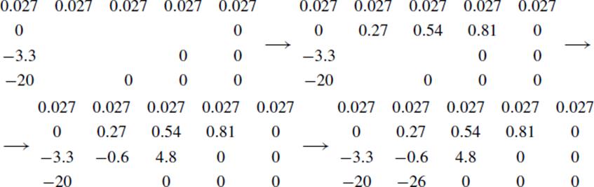
The next term y in our approximation to the roots therefore satisfies the equation 0.027y³ + 0.81y² + 4.8y − 26 = 0, and it is guaranteed to be between 0 and 10, since x = y + 10 was found to lie between 10 and 20. In fact, when y = 3, the left-hand side is −3.581, and when y = 4, it is 3.088, so that the next digit is 3. We now repeat the process.

We did the operations column-wise this time, just to show that it makes no difference whether we do it by rows or by columns. Since the next digit will be to the right of the decimal point, it makes sense to multiply the equation by 1000 to get a one-digit solution between 0 and 10. If the next correction is , it will lie between 0 and 1, and will lie between 0 and 10. If , then 0.027z³ + 10(1.053)z² + 100(10.389)z − 1000(3.581) = 0, as can be seen by multiplying the equation satisfied by by 1000, then substituting z for , z² for , and z³ for . We thus have 0.027z³ + 10.53z² + 1038.9z − 3581 = 0, and z is guaranteed to be between 0 and 10. If we had not replaced by z, we would have had to deal with fractions in making our guesses equal to 0.1, 0.2, 0.3, and so on. Once again, we find that when z = 3, the left-hand side is −368.801, and when z = 4, it is 744.808. Thus, the next digit is also 3. We now have the approximation x = 13.3. Continuing the process would reveal that .

A word of explanation is needed about the lower triangle of zeros in this method. They can be useful in getting the successive digits to the right of the decimal point if the coefficients of the original equation are all integers. Then, the equation for the next digit can be written down directly by adjoining these zeros to the coefficients one would otherwise read off.

The efficiency of this method in finding approximate roots allowed the Chinese to attack equations involving large coefficients and high degrees. Qin Jiushao (Libbrecht, 1973, pp. 134–136) considered the following problem: Three li north of the wall of a circular town there is a tree. A traveler walking east from the southern gate of the town first sees the tree after walking 9 li. What are the diameter and circumference of the town?

This problem appears to be deliberately concocted so as to lead to an equation of high degree. (The diameter of the town could surely be measured directly from inside, so that it is highly unlikely that anyone would ever need to solve such a problem for a practical purpose.) Representing the diameter of the town as x², Qin Jiushao obtained the equation³

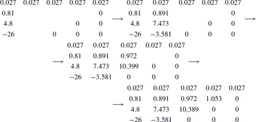
One has to be very unlucky to get such a high-degree equation. Even a simplistic approach using similar triangles leads only to a quartic equation. It is easy to see (Fig. 23.2) that if the diameter of the town rather than its square root is taken as the unknown, and the radius is drawn to the point of tangency, trigonometry will yield a quartic equation. If the radius is taken as the unknown, the similar right triangles in Fig. 23.3 lead to the quartic equation 4r⁴ + 12r³ + 9r² − 486r − 729 = 0, and since this equation has as a solution, we can divide the left-hand side by 2r + 3, getting the cubic equation 2r³ + 3r² − 243 = 0. But, of course, the object of this game was probably to practice the art of algebra, not to get the simplest possible equation, no matter how virtuous it may seem to do so in other contexts. In any case, the historian's job is not that of a commentator trying to improve a text. It is to try to understand what the original author was thinking. Probably the elevated degree is the result of having to circumvent the use of similar triangles by relying entirely on the Pythagorean theorem. (Even with that assumption, however, it is quite easy to get a quartic equation for the diameter.)

Figure 23.3 A quartic equation problem.

23.2 Later Chinese Geometry

Chinese mathematics was greatly enriched from the third through the sixth centuries by a series of brilliant geometers, whose achievements deserve to be remembered alongside those of Euclid, Archimedes, and Apollonius. We have space to discuss only three of these.

23.2.1 Liu Hui

We begin with the third-century mathematician Liu Hui (ca. 220–ca. 280), author of the Hai Dao Suan Jing mentioned in the previous chapter. Liu Hui had a remarkable ability to visualize figures in three dimensions. In his commentary on the Jiu Zhang Suan Shu he asserted that the circumference of a circle of diameter 100 is 314. In solid geometry, he provided dissections of many geometric figures into pieces that could be reassembled to demonstrate their relative sizes beyond any doubt. As a result, real confidence could be placed in the measurement formulas that he provided. He gave correct procedures, based on such dissections, for finding the volumes enclosed by many different kinds of polyhedra. But his greatest achievement is his work on the volume of the sphere.

The Jiu Zhang Suan Shu made what appears to be a very reasonable claim: that the ratio of the volume enclosed by a sphere to the volume enclosed by the circumscribed cylinder can be obtained by slicing the sphere and cylinder along the axis of the cylinder and taking the ratio of the area enclosed by the circular cross section of the sphere to the area enclosed by the square cross section of the cylinder. In other words, it would seem that the ratio is π : 4. This conjecture seems plausible, since every such section produces exactly the same figure. It fails, however, because of the principle behind Guldin's theorem: The volume of a solid of revolution equals the area revolved about the axis times the distance traveled by the centroid of the area. The half of the square that is being revolved to generate the cylinder has a centroid that is farther away from the axis than the centroid of the semicircle inside it, whose revolution produces the sphere; hence when the two areas are multiplied by the two distances, the ratio gets changed. When a circle inscribed in a square is rotated, the ratio of the volumes generated is 2 : 3, while that of the original areas is π : 4. Liu Hui noticed that the sections of the figure parallel to the base of the cylinder do not all have the same ratios. The sections of the cylinder are all disks of the same size, while the sections of the sphere shrink as the section moves from the equator to the poles. From that observation, he could see that one could not expect the ratio of the cylinder to the inscribed sphere to be the same as that of the square to the inscribed circle.

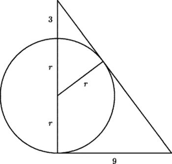
He also formed a solid by intersecting two cylinders circumscribed about the sphere whose axes are at right angles to each other, thus producing a figure he called a double square umbrella, which is now known as a bicylinder or Steinmetz solid⁴ (see Hogendijk, 2002). A representation of the double square umbrella, generated using Mathematica graphics, is shown in Fig. 23.4. Its volume does have the same ratio to the sphere that the square has to its inscribed circle, that is, 4 : π. This proportionality between the double square umbrella and the sphere is easy to see intuitively, since every horizontal slice of this figure by a plane parallel to the plane of the axes of the two circumscribed cylinders intersects the double square umbrella in a square and intersects the sphere in the circle inscribed in that square. Liu Hui inferred that the volume enclosed by the double umbrella would have this ratio to the volume enclosed by the sphere. This inference is correct and is an example of what is called Cavalieri's principle: Two solids such that the section of one by each horizontal plane bears a fixed ratio to the section of the other by the same plane have volumes in that same ratio. This principle had been used by Archimedes five centuries earlier. In the introduction to his Method, Archimedes used this very example and asserted (correctly) that the volume of the bicylinder is two-thirds of the volume of the cube in which they are inscribed.⁵ But Liu Hui's use of it (see Lam and Shen, 1985) was obviously independent of Archimedes. It amounts to a limiting case of the dissections that Liu Hui did so well. The solid is cut into infinitely thin slices, each of which is then dissected and reassembled as the corresponding section of a different solid. This realization was a major step toward an accurate measurement of the volume of a sphere. Unfortunately, it was not granted to Liu Hui to complete the journey. He maintained a consistent agnosticism on the problem of computing the volume of a sphere, saying, “Not daring to guess, I wait for a capable man to solve it.”

Figure 23.4 The double square umbrella.

23.2.2 Zu Chongzhi

That “capable man” required a few centuries to appear, and he turned out to be two men. “He” was Zu Chongzhi (429–500) and his son Zu Geng (450–520). Zu Chongzhi was a very capable geometer and astronomer who said that if the diameter of a circle is 1, then the circumference lies between 3.1415926 and 3.1415927. From these bounds, probably using the Chinese version of the Euclidean algorithm, the method of mutual subtraction, he stated that the circumference of a circle of diameter 7 is (approximately) 22 and that of a circle of diameter 113 is (approximately) 355.⁶ These estimates are very good, far too good to be the result of any inspired or hopeful guess. Of course, we don't have to imagine that Zu Chongzhi actually drew the polygons. It suffices to know how to compute the perimeter, and that is a simple recursive process: If s_n is the length of the side of a polygon of n sides inscribed in a circle of unit radius, then

Hence each doubling of the number of sides makes it necessary to compute a square root, and the approximation of these square roots must be carried out to many decimal places in order to get enough guard digits to keep the errors from accumulating when you multiply this length by the number of sides. In principle, however, given enough patience, one could compute any number of digits of π this way.

One of Zu Chongzhi's outstanding achievements, in collaboration with his son Zu Geng, was finding the volume enclosed by Liu Hui's double square umbrella. As Fu (1991) points out, this volume was not approachable by the direct method of dissection and recombination that Liu Hui had used so successfully.⁷ An indirect approach was needed. The trick turned out to be to enclose the double square umbrella in a cube and look at the volume inside the cube and outside the double square umbrella. Suppose that the sphere has radius R. The double square umbrella can then be enclosed in a cube of side 2R. Consider a horizontal section of the enclosing cube at height h above the middle plane of that cube. In the double umbrella this section is a square of side and area 4(R² − h²), as shown in Fig. 23.5. Therefore the area of the section outside the double umbrella and inside the cube is 4h².

Figure 23.5 Sections of the cube, double square umbrella, and sphere. Left: Horizontal section at height h above the midplane. Right: Vertical section through the center parallel to a side of the cube.

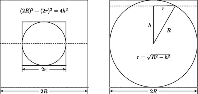
It was no small achievement to look at the region in question. It was an even keener insight on the part of the family Zu to realize that this cross-sectional area is equal to the area of the cross section of an upside-down pyramid with a square base of side 2R and height R. Hence the volume of the portion of the cube outside the double umbrella in the upper half of the cube equals the volume of a pyramid with square base of side 2R and height R. But thanks to earlier work contained in Liu Hui's commentaries on the Jiu Zhang Suan Shu, Zu Chongzhi knew that this volume was (4R³)/3. It therefore follows, after doubling to include the portion below the middle plane, that the region inside the cube but outside the double umbrella has volume (8R³)/3, and hence that the double umbrella itself has volume 8R³ − (8R³)/3 = (16R³)/3.

Since, as Liu Hui had shown, the volume of the sphere is π/4 times the volume of the double square umbrella, it follows that the sphere has volume (π/4) · (16R³)/3, or (4πR³)/3.

Problems and Questions

Mathematical Problems

23.1 Verify the solution of the problem involving three bundles of wheat, for which the solution was given above.

23.2 Use the method of the text to get the next two digits of an approximation to a root of the equation 32x³ − 24x² − 60x + 7 = 0, given that there is a root between 1 and 2. In other words, use a = 1 as a first approximation. (Remember, since you are crossing the decimal point, to carry along the extra zeros each time, as was done above.)

23.3 Find all the solutions of the cubic equation 2r³ + 3r² = 243 without doing any numerical approximation. [Hint: If there is a rational solution r = m/n, then m must divide 243 and n must divide 2.]

Historical Questions

23.4 How did Liu Hui demonstrate his geometric theorems?

23.5 What kind of algebraic problems did the Chinese solve that were different from those we have discussed from other cultures?

23.6 Why were the Chinese mathematicians undeterred by the prospect of solving equations of degree 4 and higher?

Questions for Reflection

23.7 Compare the use of thin slices of a solid figure for computing areas and volumes, as illustrated by Archimedes' Method, Bhaskara's computation of the area of a sphere, and Zu Chongzhi's computation of the volume of a sphere. What differences among the three do you notice?

23.8 The algebra developed by the Muslims and Europeans focused on expressing the solution of an equation as an algebraic expression involving the coefficients. The Chinese method, as we have seen, emphasizes finding numerical approximations to the roots. What are the advantages and disadvantages of each approach?

23.9 Since the geometric problems of finding the size of a town from measurements taken in a ludicrously indirect manner cannot have been the motive for studying cubic equations, what was the actual motive? Why was the geometry introduced at all?

Notes

1. A Latin square is a square array of symbols in which each symbol occurs precisely once in each row and precisely once in each column.

2. Besides being known to the Chinese mathematicians 600 years before Horner, this procedure was used by Sharaf al-Tusi (ca. 1135–1213) and was discovered by the Italian mathematician Paolo Ruffini (1765–1822) a few years before Horner published it. In fairness to Horner, it must be said that he applied the method not only to polynomials, but to infinite series representations. To him it was a theorem in calculus, not algebra.

3. Even mathematicians working within the Chinese tradition seem to have been puzzled by the needless elevation of the degree of the equation (Libbrecht, 1973, p. 136).

4. Named after the German-American mathematician and electrical engineer Charles Proteus Steinmetz (1865–1923).

5. Hogendijk (2002) argues that Archimedes also knew the surface area of the bicylinder.

6. The approximation was given earlier by He Chengtian (370–447), and of course much earlier by Archimedes. A more sophisticated approach by Zhao Youqin (b. 1271) that gives was discussed by Volkov (1997).

7. Lam and Shen (1985, p. 223), however, say that Liu Hui did consider the idea of setting the double umbrella inside the cube and trying to find the volume between the two. Of course, that volume also is not accessible through direct, finite dissection.