The history of mathematics: A brief course (2013)
Part VI. European Mathematics, 500-1900
Chapter 30. Sixteenth-Century Algebra
Several important innovations in algebra and computation occurred during the sixteenth and early seventeenth centuries. In Italy, cubic and quartic equations were solved. In France, a new kind of notation made it possible to discuss equations in general without having to resort to specific examples, and in Scotland the discovery of logarithms reduced the labor involved in long computations.
30.1 Solution of Cubic and Quartic Equations
In Europe, algebra was confined to linear and quadratic equations for many centuries, whereas the Chinese and Japanese had not hesitated to attack equations of any degree. The difference in the two approaches is a result of different ideas of what constitutes a solution. This distinction is easy to make nowadays: The European mathematicians were seeking a sequence of arithmetic operations, including root extractions, that could be applied to the coefficients of a polynomial equation in order to produce a root, what is called solution by radicals, while the Chinese and Japanese were seeking the decimal expansions of real roots, one digit at a time.
The Italian algebraists of the early sixteenth century made advances in the search for a general algorithm for solving higher-degree equations. We discussed the interesting personal aspects of the solution of cubic equations in Chapter 29. Here we concentrate on the technical aspects of the solution. Because the notation of the time is rather cumbersome, on this subject we are going to use some anachronistic modern notation in order to explain the solution.
The verses Tartaglia had memorized (see Chapter 28) say, in modern language, that to solve the equation x3 + px = q for x, one should look for two numbers u and ![]() satisfying
satisfying ![]() , uv = (p/3)3. The problem of finding u and
, uv = (p/3)3. The problem of finding u and ![]() is that of finding two numbers given their difference and their product; and, of course, this is merely a matter of solving a quadratic equation, a problem that had already been completely solved some 2500 years earlier. Once this quadratic has been solved, the solution of the original cubic is
is that of finding two numbers given their difference and their product; and, of course, this is merely a matter of solving a quadratic equation, a problem that had already been completely solved some 2500 years earlier. Once this quadratic has been solved, the solution of the original cubic is ![]() . The solution of the cubic has thus been reduced to solving a quadratic equation, taking the cube roots of its two roots, and subtracting. Cardano illustrated with the case of “a cube and six times the side equal to 20.” Using his complicated rule (complicated because he stated it in words), he gave the solution as
. The solution of the cubic has thus been reduced to solving a quadratic equation, taking the cube roots of its two roots, and subtracting. Cardano illustrated with the case of “a cube and six times the side equal to 20.” Using his complicated rule (complicated because he stated it in words), he gave the solution as
![]()
He did not add that this number equals 2.
30.1.1 Ludovico Ferrari
Cardano's student Ludovico Ferrari worked with him in the solution of the cubic, and between them they had soon found a way of solving certain fourth-degree equations. Ferrari's solution of the quartic was included near the end of Cardano's treatise Ars magna. Counting cases as for the cubic, one finds a total of 20 possibilities. The principle in most cases is the same, however. The idea is to make a perfect square in x2 equal to a perfect square in x by adding the same expression to both sides. Cardano gives the example
![]()
It is necessary to add to both sides an expression rx2 + s to make them squares, that is, so that both sides of
![]()
are perfect squares. Now the condition for this to happen is well known: ax2 + bx + c is a perfect square if and only if b2 − 4ac = 0. Hence we need to have simultaneously
![]()
Solving the second of these equations for s in terms of r and substituting in the first leads to the equation
![]()
This is a cubic equation called the resolvent cubic. Once it is solved, the original quartic breaks into two quadratic equations upon taking square roots and adding an ambiguous sign.
A few aspects of the solution of cubic and quartic equations should be noted. First, the problem is not a practical one. Second, the Cardano recipe for solving an equation sometimes gives the solution in a rather strange form. For example, Cardano says that the solution of x3 + 6x = 20 is ![]() . The expression is correct, but can you tell at a glance that it represents the number 2?
. The expression is correct, but can you tell at a glance that it represents the number 2?
Third, the procedure does not always seem to work. For example, the equation x3 + 6 = 7x has to be solved by guessing a number that can be added to both sides so as to produce a common factor that can be canceled out. The number in this case is 21, but there is no algorithm for finding such a number.1 For equations of this type, the algebraic procedure described by Cardano for finding x involves square roots of negative numbers. This was the first time mathematicians had encountered a need for such roots. When they occur in the solution of a quadratic equation, the roots themselves are complex numbers, making it possible to say that the equation simply has no solution. In the case of cubic equations with real coefficients, however, the algebraic procedures lead to complex numbers precisely when there are three real roots. Cardano tried to make some sense out of this case, pointing out that if one imagineda solution, it was possible to find solutions to quadratic equations that had previously been believed to have no roots. He gave as an example the problem of finding two numbers whose sum is 10 and whose product is 40, in other words, solving the quadratic equation x2 − 10x + 40 = 0, and he gave the solutions as ![]() and
and ![]() . Thus, under the influence of algebra, the stock of numbers was enlarged to include negative numbers (called false roots at first) and imaginary and complex numbers.
. Thus, under the influence of algebra, the stock of numbers was enlarged to include negative numbers (called false roots at first) and imaginary and complex numbers.
The case of three real roots came to be known as the irreducible case of the cubic. Strenuous efforts were made to avoid the use of complex numbers in this case, but careful analysis (see Chapter 37) showed that they are unavoidable. The difference between cubic and quadratic equations shows up in the fact that extracting the square root, and hence also the fourth root, of a complex number can be reduced to repeated extractions of the square roots of positive real numbers. But no such reduction exists for cube roots. When the equation (x + yi)3 = a + bi is written with real and imaginary parts separated, the result is generally a cubic equation for x having three distinct roots and a cubic equation for y having three distinct roots. Any attempt to remove complex numbers from the case when there are three real roots merely replaces one such equation with two others.
30.2 Consolidation
There were two natural ways to build on what had been achieved in algebra by the end of the sixteenth century. One was to find a notation that could unify equations so that it would not be necessary to consider so many different cases and so many different possible numbers of roots. The other was to solve equations of degree five and higher. We shall discuss the first of these here, reserving the second for Chapter 37.
All original algebra treatises written up to and including the treatise of Bombelli (to be discussed in Chapter 41) are very tiresome for the modern student, who is familiar with symbolic notation. For that reason we have sometimes allowed ourselves the convenience of modern notation when doing so will not distort the thought process involved too severely. In the years between 1575 and 1650, several innovations in notation were introduced that make treatises written since that time appear essentially modern. The symbols + and − were originally used in bookkeeping in warehouses to indicate excess and deficiencies; they first appeared in a German treatise on commercial arithmetic in 1489 but were not widely used in the rest of Europe for another century. The sign for equality was introduced by a Welsh medical doctor, physician to the short-lived Edward VI, named Robert Recorde (1510–1558). His symbol was a very long pair of parallel lines, because, as he said, “noe.2. thynges, can be moare equalle.” The use of abbreviations for the various powers of the unknown in an equation was eventually achieved, but there were two other needs to be met before algebra could become a mathematical subject on a par with geometry: a unified way of writing equations and a concept of number in which every equation would have a solution. The use of exponential notation and grouping according to powers was discussed by Simon Stevin, who was mentioned in Chapter 29. Stevin used the abbreviation M for the first unknown in a problem, sec for the second, and ter for the third. Thus (see Zeuthen, 1903, p. 95), what we would write as the equation
![]()
was expressed as follows: If we divide
![]()
we obtain
![]()
Although notation still had far to go, from the modern point of view, at least it was no longer necessary to use a different letter to represent each power of the unknown in a problem, as Leonardo of Pisa had done in his Liber quadratorum.
30.2.1 François Viète
The French lawyer François Viète (1540–1603), who worked as tutor in a wealthy family and later became an advisor to Henri de Navarre (the future king Henri IV), found time to study Diophantus and to introduce his own ideas into algebra. Viète is credited with several crucial advances in the subject. In his book Artis analyticæ praxis (The Practice of the Analytic Art) he begins by giving the rules for powers of binomials (in words). For example, he describes the fifth power of a binomial as “the fifth power of the first [term], plus the product of the fourth power of the first and five times the second, . . . .” Viète's notation was slightly different from ours, but is more recognizable to us than that of Stevin. He would write the equation A3 + 3BA = D, where the vowel A represented the unknown and the consonants B and D were taken as known, as follows (Zeuthen, 1903, p. 98):
![]()
As this quotation shows, Viète appears to be following the tedious route of writing everything out in words and to be adhering to the requirement that all the terms in an equation be geometrically homogeneous. In other words, the notion of quantity as a pure number, as opposed to a line or a plane or solid region, had not yet been introduced.
This introduction is followed by five books of zetetics (research, from the Greek word z![]() teîn, meaning seek). The mention of “roots” in connection with the binomial expansions was not accidental. Viète studied the relation between roots and coefficients in general equations. By using vowels to represent unknowns and consonants to represent data for a problem, Viète finally achieved what was lacking in earlier treatises: a convenient way of talking about general data without having to give specific examples. Consonants could be thought of as representing numbers that would be known in any particular application of a process, but were left unspecified for purposes of describing the process itself. We might call them parameters. His first example was the equation A2 + AB = Z2, in other words, a standard quadratic equation. According to Viète, these three letters are associated with three numbers in direct proportion, Z being the middle, B the difference between the extremes, and A the smallest number. In our terms, Z = Ar and B = Ar2 − A. Thus, the general problem reduces to finding the smallest of three numbers A, Ar, Ar2given the middle value and the difference of the largest and smallest. Viète had already shown how to do that in his books of zetetics.
teîn, meaning seek). The mention of “roots” in connection with the binomial expansions was not accidental. Viète studied the relation between roots and coefficients in general equations. By using vowels to represent unknowns and consonants to represent data for a problem, Viète finally achieved what was lacking in earlier treatises: a convenient way of talking about general data without having to give specific examples. Consonants could be thought of as representing numbers that would be known in any particular application of a process, but were left unspecified for purposes of describing the process itself. We might call them parameters. His first example was the equation A2 + AB = Z2, in other words, a standard quadratic equation. According to Viète, these three letters are associated with three numbers in direct proportion, Z being the middle, B the difference between the extremes, and A the smallest number. In our terms, Z = Ar and B = Ar2 − A. Thus, the general problem reduces to finding the smallest of three numbers A, Ar, Ar2given the middle value and the difference of the largest and smallest. Viète had already shown how to do that in his books of zetetics.
This analysis showed Viète the true relation between the coefficients and the roots. For example, he knew that in the equation x3 − 6x2 + 11x = 6, the sum and product of the roots must be 6 and the sum of the products taken two at a time must be 11. This observation still did not enable him to solve the general cubic equation, but he did study the problem geometrically and show that any cubic could be solved, provided that one could solve two of the classical problems of antiquity: constructing two mean proportionals between two given lines and trisecting any angle. As he concluded at the end of his geometric chapter: “It is very worthwhile to note this.” In fact, by assuming the trisection of a general angle, Viète was able to avoid the annoying complex numbers that arose in the Cardano procedure for solving x3 + px + q = 0 when it has three distinct real roots. In this case, the cubic discriminant ![]() , whose square root needs to be taken, is negative, and that is how the complex numbers arise.
, whose square root needs to be taken, is negative, and that is how the complex numbers arise.
Although complex numbers began to gain acceptance after the work of Cardano and Bombelli, attempts were still made to solve the irreducible case using only real numbers. Viète's method of doing so was the most successful. It is a transcendental solution rather than an algebraic one, since it involves the cosine function.
The classical problem of trisecting the angle reduces to a cubic equation through the trigonometric identity
![]()
This cubic equation generally has three real roots in the variable y = cos (θ/3).
Viète's technique for solving the equation x3 + px + q = 0 when there are three real roots involves “fitting” a scaled version of x to this basic equation for the cosine. Specifically, one must set ![]() . (The negative sign is necessary because the existence of three distinct real roots implies that p < 0.) The result is the equation
. (The negative sign is necessary because the existence of three distinct real roots implies that p < 0.) The result is the equation
![]()
The number y = cos (θ/3) will be a solution of this equation if the angle θ satisfies
![]()
There will be such an angle, provided that the right-hand side of this last equation lies between −1 and +1; that is, its square is at most 1. That condition amounts to 27q2/(− 4p3) ≤ 1 and can be rewritten as q2/4 + p3/27 ≤ 0. But the left-hand side of this inequality is precisely the number whose square root must be taken when following the Cardano procedure! In other words, this solution works precisely in the irreducible case. Thus, we have a nonalgebraic (transcendental) solution of the irreducible case of the cubic that does not involve any complex numbers.
30.3 Logarithms
While Viète was revolutionizing algebraic notation, the problem of simplifying laborious multiplications, divisions, root extractions, and the like, was being attacked at the same time in another part of the world and from another point of view. The connection between geometric and arithmetic proportion had been noticed earlier by Chuquet, but the practical application of this fact had never been worked out. The Scottish laird John Napier, Baron of Murchiston (1550–1617), tried to clarify this connection and apply it. His work consisted of two parts: (a) a theoretical part based on a continuous geometric model and (b) a computational part involving a discrete (tabular) approximation of the continuous model. The computational part was published in 1614. However, Napier hesitated to publish his explanation of the theoretical foundation. Only in 1619, two years after his death, did his son publish the theoretical work under the title Mirifici logarithmorum canonis descriptio (A Description of the Marvelous Rule of Logarithms). The word logarithm means ratio number, and it was from the concept of ratios (geometric progressions) that Napier proceeded.
To explain his ideas, Napier used the concept of moving points. He imagined one point P moving along a straight line from a point T toward a point S with decreasing velocity such that the ratio of the distances from the point P to S at two different times depends only on the difference in the times. (Actually, he called the line ending at S a sine and imagined it shrinking from its initial size TS, which he called the radius.) A second point is imagined as moving along a second line at a constant velocity equal to that with which the first point began. These two motions are accurately drawn in Fig. 30.1.
Figure 30.1 Geometric basis of logarithms.
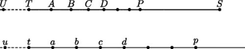
The first point sets out from T at the same time and with the same speed with which the second point sets out from t. The first point, however, slows down, while the second point continues to move at constant speed. The figure shows the locations reached at various times by the two points: When the first point is at A, the second is at a; when the first point is at B, the second is at b; and so on. The point moving with decreasing velocity requires a certain amount of time to move from T to A, the same amount of time to move from A to B, from B to C, and from C to D. The geometric decrease means that ![]() .
.
The first point will never reach S, since it keeps slowing down, and its velocity at S would be zero. The second point will travel indefinitely far, given enough time. Because the points are in correspondence, the division relation that exists between two positions in the first case is mirrored by a subtractive relation in the corresponding positions in the second case. Thus, this diagram essentially changes division into subtraction and multiplication into addition. The top scale in Fig. 30.1 resembles a slide rule, and this resemblance is not accidental: A slide rule is merely an analog computer that incorporates a table of logarithms.
Napier's definition of the logarithm can be stated in the modern notation of functions by writing ![]() ,
, ![]() , and so on; in other words, the logarithm increases as the “sine” decreases. These considerations contain the essential idea of logarithms. The quantity Napier defined is not the logarithm as we know it today. If points T, A, and P correspond to points t, a, and p, then
, and so on; in other words, the logarithm increases as the “sine” decreases. These considerations contain the essential idea of logarithms. The quantity Napier defined is not the logarithm as we know it today. If points T, A, and P correspond to points t, a, and p, then
![]()
where ![]() . For the computational table that he compiled, Napier took k = 0.9999999 = 1 − 10−7.
. For the computational table that he compiled, Napier took k = 0.9999999 = 1 − 10−7.
30.3.1 Arithmetical Implementation of the Geometric Model
The geometric model just discussed is theoretically perfect, but of course one cannot put the points on a line into a table of numbers. It is necessary to construct the table from a finite set of points; and these points, when converted into numbers, must be rounded off. Napier analyzed the maximum errors that could arise in constructing such a table. In terms of Fig. 30.1, he showed that ![]() satisfies
satisfies
![]()
These inequalities are simple to prove. The first one is obvious, since starting from time t = 0, the upper point moves from T to A with velocity that is smaller than the velocity of the point below it, which is moving from t to a. As for the second, we imagine the two motions extended into the time before the lower point was at t by the same amount of time that was required for the points to reach A and a. At that earlier time, the upper point would have been at a point U, where ![]() . Consequently
. Consequently ![]() . Since the velocity of the upper point was larger throughout this time interval,
. Since the velocity of the upper point was larger throughout this time interval, ![]() .
.
The tabular value for the logarithm of ![]() can be taken as the average of the two extremes, that is, as
can be taken as the average of the two extremes, that is, as ![]() , and the relative error will be very small when TA is small.
, and the relative error will be very small when TA is small.
Napier's death at the age of 67 prevented him from making some improvements in his system, which are sketched in an appendix to his treatise. These improvements consist of scaling in such a way that the logarithm of 1 is 0 and the logarithm of 10 is 1, which is the basic idea of what we now call common logarithms. These further improvements to the theory of logarithms were made by Henry Briggs (1561–1630), who was in contact with Napier for the last two years of Napier's life and wrote a commentary on the appendix to Napier's treatise. As a consequence, logarithms to base 10 came to be known as Briggsian logarithms.
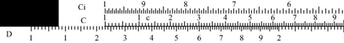
Portions of the C, D, and CI scalesof a slide rule. Adjacent numbers on the C and D scales are in proportion, sothat 1 : 1.23 : : 1.3 : 1.599 : : 1.9 : 2.337. Thus, the position shownhere illustrates the multiplication 1.23 · 1.3 = 1.599, thedivision 1.722 ÷ 1.4 = 1.23, and many other computations. Some visual error is inevitable. The CI (inverted) scale gives the reciprocals ofthe numbers on the C scale, so that division can be performed as multiplication, only using the CI scale instead of the C scale. Decimal points have to beprovided by the user.
30.4 Hardware: slide rules and calculating machines
The fact that logarithms change multiplication into addition and that addition can be performed mechanically by sliding one ruler along another led to the development of rulers with the numbers arranged in proportion to their logarithms (slide rules).
30.4.1 The Slide Rule
When one such scale is slid along a second, the numbers pair up in proportion to the distance slid, so that if 1 is opposite 5, then 3 will be opposite 15. Multiplication and division are then just as easy to do as addition and subtraction would be. The process is the same for both multiplication and division, as it was in the Egyptian graphical system, also based on proportion. Napier designed a system of rods for this purpose. The twentieth-century refinement of this idea is the slide rule.
A variant of this linear system was a system of sliding circles. Such a circular slide rule was described in a pamphlet entitled Grammelogia written in 1630 by Richard Delamain (1600–1644), a mathematics teacher living in London. Delamain urged the use of this device on the grounds that it made it easy to compute compound interest. Two years later the English clergyman William Oughtred (1574–1660) produced a similar description of a more complex device. Oughtred's circles of proportion, as he called them, gave sines and tangents of angles in various ranges on eight different circles. Because of their portability, slide rules remained the calculating machine of choice for engineers for 350 years, and improvements were still being made in them in the 1950s. Different types of slide rule even came to have different degrees of prestige, according to the number of scales incorporated into them.
30.4.2 Calculating Machines
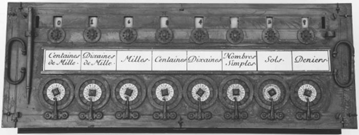
Slide rule calculations are floating-point computations—that is, the user has to keep track of the location of the decimal point—with limited precision and unavoidable roundoff error. When computing with integers, we often need an exact answer. To achieve that result, adding machines and other digital devices have been developed over the centuries. An early design for such a device with a series of interlocking wheels can be found in the notebooks of Leonardo da Vinci (1452–1519). Similar machines were designed by Blaise Pascal (1623–1662) and Gottfried Wilhelm Leibniz (1646–1716). Pascal's machine was a simple adding machine that depended on turning a crank a certain number of times in order to find a sum. Leibniz used a variant of this machine with a removable set of wheels that would multiply, provided that the user kept count of the number of times the crank was turned.
A replica of Pascal's addingmachine constructed by Roberto Guatelli (1904–1993). Copyright© Richard Marks. Courtesy of The Computer HistoryMuseum.
Problems and Questions
Mathematical Problems
30.1 Verify (using a calculator) that the expression given for a root of x2 + 6x = 20 really is the number 2. If you didn't have a calculator, how would you demonstrate this fact convincingly to someone?
30.2 Solve the problem that Viète solved, finding all three of the numbers A, Ar, and Ar2, given that the middle term Ar is 15 and the difference between the largest and smallest is 40.
30.3 Find ![]() by first finding the logarithm of 53, dividing it by 5, and taking the antilogarithm of the result. Use a calculator to do it in two ways, first with the LOG function, so that the antilogarithm of x is 10x; then use the LN function, so that the antilogarithm of x is ex. Finally, check your work by computing 531/5 = 530.2 directly on the calculator.
by first finding the logarithm of 53, dividing it by 5, and taking the antilogarithm of the result. Use a calculator to do it in two ways, first with the LOG function, so that the antilogarithm of x is 10x; then use the LN function, so that the antilogarithm of x is ex. Finally, check your work by computing 531/5 = 530.2 directly on the calculator.
Historical Questions
30.4 Who were the main figures involved in the solution of cubic and quartic equations, and what did each of them do?
30.5 What contributions to algebra are due to François Viète?
30.6 In what way were logarithms an improvement on prosthaphæresis? Are there any situations in which one might prefer prosthaphæresis?
Questions for Reflection
30.7 The general problem of solving a quadratic equation with complex coefficients reduces through the quadratic formula to the extraction of one square root (which may be the square root of a complex number) followed by simple additions or subtractions and division. Extracting the square root of a complex number a + bi amounts to solving simultaneously the equations x2 − y2 = a and 2xy = b, and these can be reduced to taking two square roots of positive real numbers. Hence there exists a purely real procedure for solving any quadratic equation when the roots are real. Taking the cube root of a + bi, however, means simultaneously solving x3 − 3xy2 = a, 3x2y − y3 = b. In general, there are three pairs of real numbers (x, y) that will satisfy these two equations simultaneously, but finding them, as noted above, requires introducing complex numbers yet again. In what sense, then, has the general cubic equation been solved?
30.8 Why was the introduction of special letters to denote constants and variables an important advance in algebra?
30.9 We have seen that multiplication and division can be reduced to addition and subtraction in two different ways, namely prosthaphæresis and logarithms. What can you infer from this fact about the relation between trigonometric, logarithmic, and exponential functions?
Note
1. There is an algorithm for finding all rational solutions of an equation with rational coefficients; but when the roots are irrational, this problem remains.