Mathematics for the liberal arts (2013)

Part I. MATHEMATICS IN HISTORY

Chapter 4. CALCULUS

4.3 Tangent Line to a Curve

If we think about the process we developed in Section 4.2, each time we chose a time interval and computed the average velocity of the pencil over the interval, we were finding a value that looked something like

Considering the problem geometrically (looking at the graph of what we are doing), we can see that the key to the whole process is slopes. Since slope is the ratio of the change in the y-coordinates (the rise) to the change in the t-coordinates (the run), we can write slope as Δy/Δt. (The Greek letter delta, Δ, stands for change.) Each of these average velocities is the slope of some line intersecting the height function at two points. See Figure 4.2.

We saw that finding the instantaneous velocity amounted to a limiting problem where Δt, which we called by the name h, was allowed to get closer and closer to zero. In the picture, we interpret this as a question about the slopes of lines that intersect a function when the points of intersection are brought closer and closer together. Each average velocity for the pencil is the slope of some line through the curve, so if we want to know about the (instantaneous) velocity of the pencil, we can focus our attention on slopes of lines.

A tangent line to a curve is a line that touches the curve in just one point, and closely approximates the curve near that one point. In Figure 4.3, a tangent line is drawn touching the curve where t = 1/2. Notice that the tangent line looks very much like the limit of the lines in Figure 4.2 when Δt approaches zero.

Figure 4.4 shows a general curve and a tangent line to the curve at a point P on the curve.

To find tangent lines in general, we use our experience with instantaneous velocities for inspiration. To find the tangent line at P in Figure 4.5, we begin by putting a second point Q on the curve somewhere nearby. We can put Qpretty much any where on the curve to start out, though often you’ll pick somewhere near P. The line through P and Q is called a secant line.

Figure 4.2 Average velocities are slopes of lines.

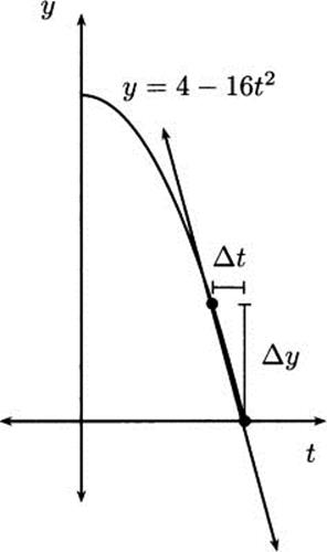
Figure 4.3 A tangent line is the key to instantaneous velocity.

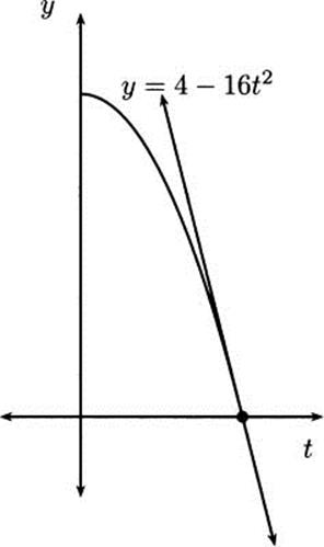
Figure 4.4 A curve and its tangent line.

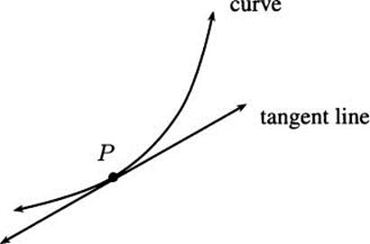
Figure 4.5 Tangent lines are derived from secant lines.

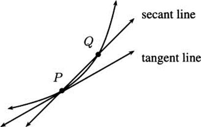
Now, if Q gets closer and closer to P (which is what happened when we observed our pencil over shorter and shorter time intervals), then the secant line through P and Q becomes a better and better approximation to the tangent line at P. If we can make Q coincide with P, by using a limiting process, then the secant line will “become” the tangent line at P. This is good for us, since the slope of the tangent P is going to tell us how fast our pencil hits the floor.

In the following examples, we will refer to P (the point where the tangent line touches the curve) as the base point. We will refer to Q as the second point.

The method of using a limiting process of secant lines to find a tangent line was discovered by Pierre de Fermat (1601–1665). It was expanded upon by the two discoverers of calculus, Isaac Newton (1642–1727) and Gottfried Wilhelm von Leibniz (1646–1716).

EXAMPLE 4.1

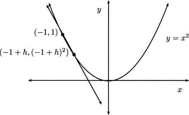
We will find an equation of the tangent line to the parabola y = x² at the point (–1, 1). The base point is (–1, 1). We take the second point to be (–1 + h, (–1 + h)²), where h is an arbitrary nonzero number. In Figure 4.6, h is positive, so the second point is to the right of the first point. But h could just as well be negative, with the second point to the left of the base point. The calculations work the same either way.

Figure 4.6 Tangent to y = x².

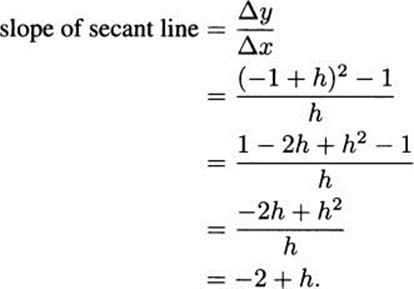
When h diminishes to 0, we obtain the slope of the tangent line:

We have a slope, –2, and a point, (–1, 2), so we can use the point-slope form of a line, y – y₀ = m(x – x₀), to describe the tangent. Thus, an equation of the tangent line to y = x² at the point (–1, 1) is

If we want to solve this equation for y to put the line in the more familiar y = mx + b form, we can:

EXAMPLE 4.2

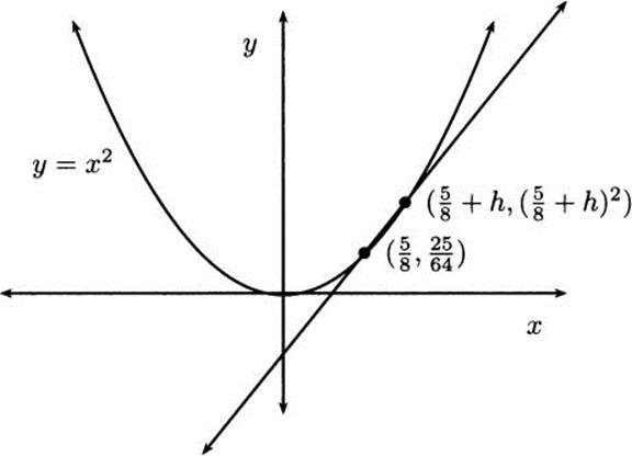
Let’s find an equation of the tangent line to the parabola y = x² at the point (see Figure 4.7).

Figure 4.7 Tangent to y = x² at .

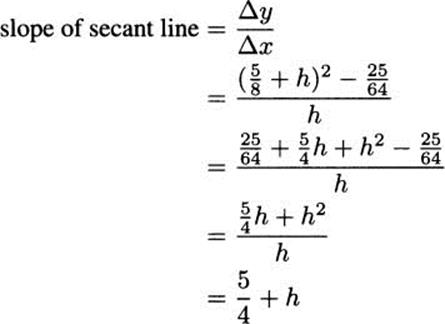
When h diminishes to 0, we obtain the slope of the tangent line:

Using the point-slope form again, an equation of the tangent line is

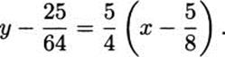
Looking over the last two examples, we see that the slope of the tangent line to the curve y = x² at the point (–1, 1) is –2, and the slope of the tangent line to the same curve at the point is . In both cases, the slope of the tangent line is double the value of the x coordinate. Let’s use the next example to show that this is always the case for the curve y = x².

EXAMPLE 4.3

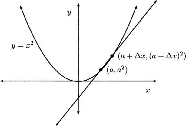
Let’s find the slope of the tangent line to the parabola y = x² at the point (a, a²), where a is an arbitrary number (Figure 4.8). Based on our previous work, we expect that our answer is going to be 2a.

This time, for variety, we choose to write Δx for h.

Figure 4.8 Finding the slope at an arbitrary value a.

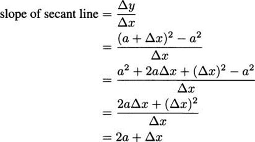
When Δx diminishes to 0, we obtain the slope of the tangent line:

Notice that if we let a = – 1, then we find the slope of the tangent line at (–1, 1), and we get the same answer, –2, as we got in Example 4.1. If we let a = 5/8, we get the same answer, 5/4, that we got in Example 4.2.

EXERCISES

4.6 Use the secant line method to find an equation of the tangent line to the parabola y = x² at the point (3,9).

4.7 Use the secant line method to find an equation of the tangent line to the parabola y = x² at the point (–4, 16).

4.8 Use the secant line method to find an equation of the tangent line to the parabola y = 4 – 16t² at the point (0.25, 3).

4.9 Find the slope of the tangent line to the parabola y = 4 – 16t² at an arbitrary point (a, 4 – 16a²). The slope of this tangent corresponds to the velocity of our falling pencil in Section 4.2. Use this slope to determine the velocity of the pencil when t = 0.0, 0.1, 0.2, 0.3, 0.4, and 0.5 seconds.

4.10 Find the slope of the tangent line to the parabola y = 16 – 16t² at an arbitrary point (a, 16 – 16a²). The slope of this tangent corresponds to the velocity of a pencil dropped from a height of 16 feet. Use this slope to determine the velocity of the pencil when t = 0.0, 0.25, 0.5, 0.75, and 1.0 seconds.

4.11 Find the slope of the tangent line to the parabola y = 4–2.65t² at an arbitrary point (a, 4–2.65a²). The slope of this tangent corresponds to the velocity of a pencil dropped from a 4 foot desk on the Moon. Use this slope to determine the velocity of the pencil when t = 0.0,1, and 1.2286 seconds.

4.12 If your home were on Mars, the height function of a pencil dropped from a 4 foot desk would be the parabola y = 4 – 6.12t².

a) Set y = 0 to find the time t when your pencil strikes the floor.

b) Find the slope of the tangent line to the height function at an arbitrary time a.

c) Find the velocity that the pencil strikes the floor.

d) Compare your answer from part (c) to pencils on the Earth or Moon.