Mathematics of Life (2011)

Chapter 9. Taxonomist, Taxonomist, Spare that Tree

Anyone who visits a zoo quickly notices that some animals are more alike than others. Lions, tigers, leopards and cheetahs are all variations on a basic ‘cat’ design; polar bears, brown bears and grizzly bears are all bears; wolves, foxes and jackals are dog-like, and so on. Our best explanation of these resemblances, along with misleading exceptions such as dolphins resembling sharks, is evolution. However, the similarities were developed into a systematic classification of life on Earth, long before Darwin devised the first credible theory for their occurrence. One of the first steps in the development of any branch of science is to find a way to organise the wealth of observations that nature presents to us, and this is especially necessary in biology, because of the vast diversity of life.

As we’ve seen, the first important step in this direction was made by Linnaeus, with his ambitious scheme to classify not just animals, but plants and minerals as well. He was not the first to try to bring some kind of order into such matters, and some of his terminology goes back to Aristotle, but his method was the first to be widely adopted.

We can represent the eightfold hierarchy of taxonomic ranks diagrammatically. Life subdivides into three domains; each domain subdivides into a number of separate kingdoms, and so on. Mathematically, a series of subdivisions of this type has the structure of a tree – a diagram with repeated branchings (see Figure 18). The trunk of the tree is Life; this splits into three major limbs, the domains, which are eukaryotes, prokaryotes and archaea. Each domain splits into kingdoms: for example the eukaryote domain divides into animalia, plantae, fungi, amoebozoa, chromalveolata, rhizaria and excavata. The first two are animals and plants, the third is what it appears to be, and you can look the fancy ones up if you want to know what they are. Then animalia divides into a large number of phyla – so large that it is normal to first split it into subkingdoms, then these split into superphyla, and finally those split into phyla.

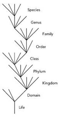
Fig 18 Classification scheme drawn as a tree (most branches not shown).

One of the reasons why these further subdivisions have arisen is that, over time, we have discovered vastly more species than were known when Linnaeus first began to catalogue nature’s diversity. But the growing complexity of the system of nomenclature, and the arguments that often accompany this process, also indicate that the rich panoply of life does not easily fit into any preassigned scientific straitjacket. Many modern biologists think that this system is no longer adequate to describe the complicated interrelationships found in living creatures, which is probably correct, but it does suffice to label them, and it is convenient, traditional and comprehensible by humans – unlike the suggested replacements.

Linnaeus’s classification scheme made it possible to establish, fairly definitively, whether any new-found organism was a genuinely new species or one that was already known. It also had a seductive allure, structuring all Earth’s life forms into a single Tree of Life, one of the enduring and iconic evolutionary images. This captures, in diagrammatic form, the relationships among present-day species and their evolutionary ancestors. Ernst Haeckel produced many wonderful evolutionary trees, in a somewhat baroque style of representation; precursors go back to Darwin’s notebooks and a diagram in the Origin. Darwin, realising that he lacked sufficient data, did not commit himself to a single origin. But it is clear that he did not expect dozens of independent origins for various types of creature. A majestic tree, with bifurcating boughs, branches, twigs and twiglets, provides a vivid metaphor for the idea that all living creatures are related, and that there was a single origin of life (see Figure 19). Or possibly a small number of separate origins, which would lead to several disconnected trees.

Part of the image’s appeal is our familiarity with ‘family trees’, especially of royal families. Today there are genealogical websites where you can research your family’s history and draw up a tree showing your parents, grandparents, siblings and other close relatives. This familiarity makes us think we understand family trees, and leads us to view the Tree of Life as something similar. However, diagrams like this can cause confusion. Do the branches represent species, or relationships among species? Do they represent species that exist today, or ones that used to exist and are now found only as fossils? When evolutionary explanations came into fashion, the distinction became vital, but was often ignored. For example, the jibe ‘Which ape was your grandfather, Mr Darwin?’ assumed that today’s apes could be humanity’s past ancestors. This isn’t what Darwin was suggesting, and in any case it’s impossible unless someone invents a time machine.

Is a tree an appropriate metaphor for evolutionary divergence?

When species split through evolution, a process known as speciation, a single species typically becomes two. It is difficult not to speak of this process as ‘branching’, and just like the branches of a real tree, species split repeatedly. Trees have always loomed large in humans’ daily life, so the metaphor is a natural one.

However, it can be pushed too far. Haeckel’s tree diagrams resemble real, though artistically stylised, trees. His artist even gave them bark and roots. And he made the trunk thicker than the branches that split off from it, which is distinctly misleading if, as seems natural, the thickness of a branch represents the abundance of the corresponding species. The real Tree of Life starts with a thin trunk, and many branches are thicker than the trunk from which they grow, as some species become wildly successful and populate the planet in huge numbers. Haeckel also drew his trees so that ‘higher up’ meant ‘more advanced’. Superficially, this also correlates with ‘more recent’, until you realise that branches corresponding to, say, bacteria have to reach all the way to the very top of the tree, and in Haeckel’s pictures they don’t. For such purposes, a better representation looks less like a real tree, though it still has the characteristic branching behaviour (see Figure 20).

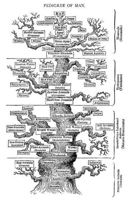
Fig 19 Haeckel’s pedigree of Man, 1906.

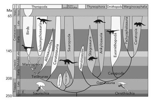
Fig 20 A less misleading Tree of Life showing how birds evolved from dinosaurs.

Mathematicians have their own concept of ‘tree’, and it too is a metaphor, one that has been enshrined as a specific concept: a diagram in which dots, which can be omitted when the junctions are obvious, are connected by lines, and branches cannot reconnect. This is equivalent to the requirement that no set of edges forms a closed loop. Mathematical trees appear in a more modern realisation of the ‘tree’ metaphor, known as a cladogram, which comprises little more than the branch points and their timing.

Figure 21 shows a cladogram for the domestic dog and various evolutionary relatives. Note that time runs from left to right here, whereas it runs from bottom to top in Figures 19 and 20. Both conventions are common. The black bear is included deliberately as an ‘outgroup’, expected on many grounds to be far less closely related to dogs than any other species in the diagram. This is a technical device to permit reliable comparisons, and also a quick-and-dirty test of the end result: if dogs turn out to be more closely related to bears than jackals, we would suspect something had gone wrong and re-examine our data. We expect the outgroup to determine the base – the trunk – of the tree.

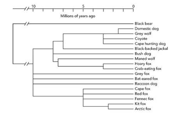
Fig 21 Cladogram for the domestic dog.

Cladograms are assembled by computer analysis of similarities and differences between species. These might be lists of characters, such as ‘four-legged’ or ‘has canine teeth’. The timings here are imprecise and give little more than the ordering of successive splits. But it is becoming increasingly common to use lists of alleles (gene variants) or even DNA sequences related to genes, with the timing inferred from the ‘genetic clock’, the average rate at which mutations occur.

I could say a lot about all this, but I don’t want to get sidetracked into a technical area. Suffice it to say that nothing here is guaranteed to be 100% accurate. In particular, the resulting tree is the one that is most likely to fit the data, according to various more or less arcane measures of likelihood. This does not mean that it is definitely an accurate reconstruction of the actual pattern of evolutionary descent. Of course, if more independent data can be collected and a given tree structure survives, that increases the likelihood that it is correct. A cladogram is a diagram encoding a long list of statements like ‘according to the following criteria, a crab-eating fox is more like a maned wolf than it is like a coyote’.

Cladistics was introduced by the entomologist Willi Hennig in 1966, in his book Phylogenetic Systematics. As the title suggests, he wanted to make the classification of organisms more systematic, avoiding the often subjective decisions of traditional taxonomy. For Hennig, the basic unit of classification was the clade, which consists of an ancestral organism along with all its evolutionary descendants. In a tree diagram, a clade is a single branch together with everything that grows from it.

Conventional cladistics (the construction of cladograms) starts with the assumption that what we are seeking is a tree. If the real pattern of descent is not tree-like, the method will find a tree anyway. This is not as bad as it might seem, because a tree is usually the sensible option. With simple modifications to the method, the tree structure itself can be tested.

The number of possible trees grows rapidly with the number of species. There are, for example, 105 distinct trees for 5 species, and 34,459,425 for 10 species. There is even a formula: for n species, the number of trees is 1 × 3 × 5 × 7 × ...× (2n-3). This is superexponential growth – faster than any power of a specific number. Somehow, the ‘best’ tree has to be chosen from among all these possibilities. Naturally, there are many different definitions of ‘best’, and for any such definition, there are many different mathematical schemes for finding it.

The methods used have become very technical. They are carried out using computers, because the amount of data, and the complexity of the calculations, are greater than an unaided human can handle. But in the early days of cladistics, a lot was done by hand. In simple terms, the technique involves three steps: collect data on the organisms concerned, think about suitable cladograms, choose the best of these. The data take the form of lists of specified characters, so that for bird species it might be things like width of beak, length of beak, colour of feathers, size of feet. Once DNA sequencing became practical (initially for short sequences such as mitochondrial DNA) the data collected usually include DNA, and today many practitioners use nothing else.

The mathematical task is now to find which tree fits the data best. This requires defining some number, known as a metric, that quantifies how closely the tree agrees with the data. Two species with similar data should be close together in the tree – that is, their common ancestor should not be many branches back. Species with less similar data should be separated by more branches. The actual recipes are not as vague as this outline might suggest. Also, there are well-established guidelines for avoiding a choice of characters that might be misleading – something that arises in many different organisms for reasons that do not relate to common ancestry. The shapes of sharks and dolphins, with the same sort of tail and triangular dorsal fin, are examples.

Suppose for example, that we are trying to sort out the relationships among four species of cat: (domestic) cat, leopard, tiger and cheetah. To keep ourselves honest we include an outgroup: snail. We select four characters (way too small for a serious analysis, but it will show how the method works), and tabulate these against the five species, using 1 for ‘yes’ and 0 for ‘no’, as in Table 6.

As a measure of how closely different species are related (which is the opposite of ‘distance’, so minimising distance is the same as maximising closeness), we could use the number of entries in the matrix that they have in common. For example, cat and leopard agree on whiskers and purr, but not on spots and big, so the distance is 2. In this case the small quantity of data lets us tabulate all possible closenesses, as in Table 7.

Next, we apply some heuristics, a fancy word for ‘informed guesswork’. The closest any two species get is 3, and that is for all four types of feline, so we guess that the four types of cat are more closely related to each other than to the snail. This places the snail at the bottom of the tree, where it belongs. Next, the cat is closely related to the tiger and cheetah (closeness 3), but less closely to the leopard (closeness 2), so we expect to find these three at the top of the tree. So we make the cheetah the first species to branch away from snail. Among cat, leopard and tiger, the first two are closer to the cheetah, so we make the tiger branch before the other two do.

Table 6 Four characters in five species.

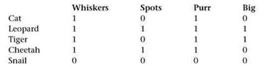
Table 7 Closeness of the five species.

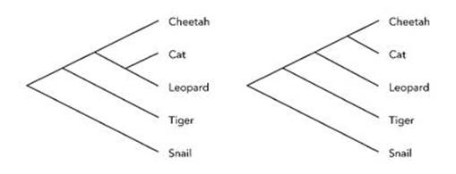
Fig 22 Two candidate cladograms.

At this point there are two different ways to complete the tree, illustrated in Figure 22: either cat and leopard both branch from the line leading to cheetah, and then split, or cheetah and cat branch from leopard.

In the first picture, cat is closer to leopard than to cheetah, but actually it’s closer to cheetah than to leopard, which is what the second picture shows. So we plump for the second tree. But this tree is not the answer: just the first step in finding it. If we had made comparisons in a different order, for instance, we might have been led to a different tree. To complete the construction of the best-fitting tree, we therefore need some measure of how well the overall tree fits the data. Then we look at variations on our candidate tree – say, swapping leopard and tiger – and see whether they do better. We should also swap snail with, say, tiger, to make sure that our outgroup really is an outgroup, otherwise there’s no point in including it in the first place.

To find the best tree, we need to work out the sums for all possible trees. The formula tells us that there are 15 of these, so the calculation is feasible, but in practice we work with many more characters, and a different approach is needed, described below. Since this example is much too simple-minded anyway, I won’t take the analysis any further, but the general gist of the method should now be apparent.

Because the number of possible trees grows very rapidly with the number of species, it is not possible in practice to calculate the best-fitting tree with perfect accuracy. However, many methods exist to find a tree that fits almost as well as the theoretical best one. They are borrowed from an area of mathematics known as optimisation, often used in industry and economics.

The construction of a plausible cladogram might go like this. First, the cladist uses their experience, or other so-called heuristic methods, to write down a small number of trees that are expected to be close to optimal. These are input into a computer running suitable software, and the computer randomly generates trees that are slight modifications of the initial guesses. It then calculates the metric – how good the fit is – and sees which of the modified trees performs best. The process is now repeated, with random variants of this new tree, and continues until no random modification makes the tree any better.

In an analogy, imagine that the metric represents height in a landscape. The best-fitting tree corresponds to the highest point in the entire landscape. However, there may be several hills, each with its own local peak; only one of those will be the highest point around. So the idea is to choose a few plausible starting points, and then search randomly near those to see if any path leads upwards. If so, wander a little way up the path and repeat the search. The main problem with such methods is that if your initial guess isn’t a good one, you may get stuck on a hill that is not the highest one around. Searching nearby won’t improve the outcome; you have to search further afield. There are sensible ways to do that, but none of them are foolproof.

There is also no guarantee that the tree obtained by this method is actually the precise evolutionary tree of the species involved. But we can be fairly confident that if the tree shows two species to be very closely related, or very distantly related, then much the same holds for the genuine evolutionary tree. We can be very confident if different data, analysed by different methods, lead to similar results.

All very well, but ... How sensible is it to model evolution as a tree?

In Wonderful Life, Stephen Jay Gould discussed the diverse softbodied creatures found in fossils from the Burgess Shale, a deposit of rock strata in Canada. These deposits, and the fossils within them, come from the time of the Cambrian explosion, a sudden burst of diversity that led to the evolution of many different, highly complex creatures. Unusually, the fossils preserve many soft features that would normally have rotted away. According to Gould’s interpretation, the evolutionary descent of the Burgess Shale fossils looks more like a bushy savannah than a single tree. However, bushes corresponding to species that have all become extinct do not reach to the present day, and so cannot be reconstructed from present-day data.

In fact, Gould suggested that the Burgess Shale fauna contained more phyla – one of the largest units into which life forms are classified – than currently exist. Humans, for example, belong to the phylum of chordates, creatures that develop a notochord as an embryo. He went on to deduce that the evolution of humanity involved a random ‘accident’ at the time of the Cambrian explosion. Pikaia, which among the Burgess Shale fauna is the best candidate ancestral species for all chordates, left surviving descendants. Anomalocaris, Opabinia, Nectocaris, Amiskwia and various other organisms, each representing a distinct (and now extinct) phylum, did not – even though all these creatures were happily coexisting, and there seems to be no good reason to expect any one of them to survive and the others to die out.

It now seems that Gould inadvertently exaggerated the differences among the fossils he considered, and many are in fact related to existing creatures, contrary to what he thought. However, it is also true that many equally baffling Burgess Shale fossils have not yet been analysed at all, so Gould’s theory might yet be revived. At any rate, if you look for a tree you will find a tree, so for some questions it makes sense not to start by assuming that a tree exists.

In a genetic interpretation, the Tree of Life represents how genes pass from (organisms in) ancestral species to (organisms in) their descendant species. However, there is a second way for genes to be transferred between organisms. It was discovered in 1959 by a Japanese team, which discovered that antibiotic resistance could be transmitted from one species of bacterium to a different species.¹ This phenomenon is known as horizontal (or lateral) gene transfer, whereas the conventional transmission of genes to descendants is called vertical transfer. The terms are derived from the usual tree diagram of evolution, with time running vertically and species-type horizontally, and have no other significance.

It soon became apparent that horizontal gene transfer is widespread among bacteria, and not uncommon in single-celled eukaryotes. This changes the paradigm for evolution among such creatures, because it introduces a different way for genomes to change. The classical concept of genetic changes arising through mutations (including deletions, duplications and reversals, as well as point mutations) in the genome of an organism in a single species must be broadened to allow the insertion of segments of DNA from a different species altogether. There are three main mechanisms for such transfer: the cell may incorporate alien genetic material through its own workings, alien DNA may be brought in by a virus, or two bacteria may exchange genetic material (‘bacterial sex’).

There is also some evidence that multi-celled eukaryotes may have been the recipients of horizontal gene transfer at some stage in their evolutionary history. The genomes of some fungi, in particular yeast, contain DNA sequences derived from bacteria. The same goes for a particular species of beetle that has acquired genetic material from Wolbachia bacteria, which live inside the beetle in a state of symbiosis. Aphids contain genes from fungi which let them manufacture carotenoids. The human genome includes sequences derived from viruses.

These effects certainly change our view of how genetic changes, one of the driving forces behind evolution, can occur. They imply that many creatures’ genetic ancestry involves more than their obvious evolutionary ancestors. A number of biologists have argued that this forces us to abandon the Tree of Life metaphor. Scientifically, this poses no great obstacles: the Tree of Life is not sacred, and if the evidence indicates that it is wrong, it should be discarded. Our view of evolution would then be different – at least in so far as the standard metaphor goes – but science often progresses by revising previous ideas. So does horizontal gene transfer wreck the Tree of Life metaphor?

At first sight the answer seems to be ‘yes’. Horizontal gene transfer can introduce closed loops, by linking two distinct branches of the usual tree. And then it’s not a tree.

However, the branches in Haeckel’s Tree of Life, and in cladograms, represent how species branch, either historically or conceptually. They don’t represent individual organisms. Horizontal gene transfer moves a snippet of DNA from one organism to another. So this new link is not a branch on the species tree. A cow becomes a cow with a bit of alien DNA, but it’s still a cow. Of course, the alien DNA affects what it might evolve into in future, but that comes later, if at all.

In a diagram with conceptual branches showing how organisms or species are connected by changes to their DNA, horizontal gene transfer does throw in some extra connections that spoil the tree structure. But this doesn’t mean that the original Tree of Life metaphor was wrong. It just means that we’re talking about a different metaphor.

In short, horizontal gene transfer has no effect on the Tree of Life for species. It has a small effect on the tree for organisms, and a bigger effect on the tree for DNA. There is perhaps one exception to these statements: when the species are bacterial or viral. Then horizontal gene transfer is so common that even the concept of a species is questionable.

Speciation, considered for individuals, is probably a very complicated intermingling of edges. Representing the speciation event as a simple branch point almost certainly oversimplifies the process, and leads to questions and distinctions that may not be appropriate (such as ‘exactly when did the two species split’?). Some complex system models of speciation introduced by Toby Elmhirst under the name BirdSym exhibit very complex cascades of changes in phenotype during speciation events. The pictures look more like braided rivers than simple branch points.

Might there be not one Tree of Life, but several? Darwin left this possibility open in the Origin. The general idea of evolution would not be greatly affected, whatever the answer, but there is an evolutionary reason to prefer a single tree. Once life gets going – by whatever method – it reproduces, and this makes any subsequent independent origin unlikely to get very far. The new kids on the block have to compete with those that are there already, who have an advantage because they have become pretty good at playing the evolutionary game. So we would expect a single origin, and would need new ideas to explain a multiple one.

In 2010 Douglas Theobald used methods from cladistics to test this hypothesis, known as ‘universal common ancestry’, and the results came down firmly in favour of a common ancestry for all present-day life.² The word used here is ‘ancestry’, not ‘ancestor’, with good reason. Theobald’s model permits the last universal common ancestor to be a population of different organisms, with different genetics, living at different times. His method involves the amino acid sequences of 23 proteins, found across all three domains of life – archaea, prokaryotes and eukaryotes. You can think of them as molecular probes that cover the entire range of living creatures, and go way back into deep time. Having chosen the proteins, the next step is to calculate evolutionary trees and sets of several trees. The final step is to compare how likely these results are, given the data.

Theobald compared a single tree, perhaps with additional horizontal gene transfer, with (say) two trees, which may or may not be linked together by horizontal gene transfer. His result is dramatic: a single tree is about 10^2,860 times as likely as two or more trees (see Figure 23). To put this in perspective, it is like randomly shuffling a pack of cards and finding that the cards are arranged in perfect order, ace to king for spades, hearts, clubs and diamonds . . . and repeating this 42 times.

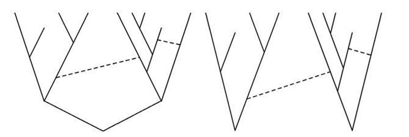
Fig 23 A unique Tree of Life like the left-hand diagram is 10^2,860 times as likely as a multiple tree like the right-hand one. Dashed lines represent horizontal gene transfer and are not part of the tree.