Mathematics of Life (2011)

Chapter 11. Hidden Wiring

Compared with most other animals, we have unusually large brains. We’re very proud of our brains, because they are the source of human intelligence, which by any reasonable definition is greater than that of almost all other creatures (though I do wonder about dolphins). However, intelligence can’t be just a matter of brain size, absolute or relative. Some animals have bigger and heavier brains than we do, and some animals have brains whose weight, in proportion to that of their bodies, is greater than ours. So brain size or weight alone seems not to imply intelligence, and neither does the relative brain size or weight (see Figure 33).

In fact, our big brains may not be as unusual as has previously been assumed. Suzana Herculano-Houzel and colleagues at the Laboratory of Comparative Neuroanatomy in Rio de Janeiro have analysed brain size in numerous species, finding that our brains are about the size you would expect in a large primate.¹ As far as brain size goes, we are no more than scaled-up monkeys.

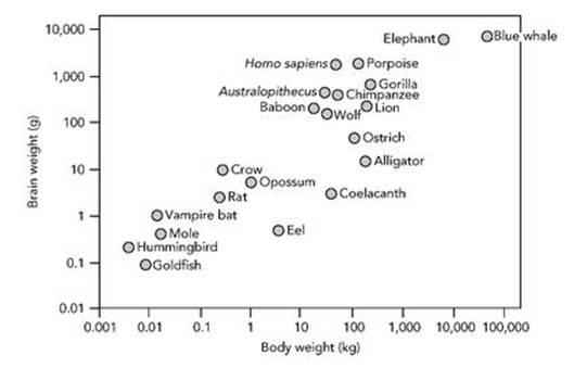
Fig 33 How brain weight relates to body weight.

However, monkeys are smart. A lot smarter than many creatures with brains the same size. In many types of animal, larger brains also have larger nerve cells, but in primates, nerve cells remain the same size no matter how big the brain. So a monkey brain has a lot more nerve cells than, say, a rodent brain of similar physical size.

What matters is not how big a brain you have, but what it can do and how you use it.

In ancient times, the function of the brain was a mystery. When the Egyptians mummified their pharaohs, they carefully removed the liver, lungs, kidneys and intestines, putting them in so-called canopic jars, so that the king would be able to use these vital organs in the afterlife. But they scraped out the brain by opening a hole into the skull through the back of the nose, stirred the brain until it turned to mush, drained it out and threw it away. They clearly thought that the king would not need his brain in the afterlife, and their reason was that it didn’t seem to do anything.

On the other hand, like all cultures of the period, they knew that if someone’s head was caved in with a club, in battle, then they would die. One of the favourite depictions on temple walls was a ‘smiting scene’ in which the king clubbed his enemies with a mace. So they presumably realised that you needed an intact head to survive, but discounted the brain because it didn’t appear to have any useful function. It was just padding for the head.

The human brain is a very complicated organ, made from nerve cells: special types of cell that link together into chains and networks and send signals to one another. A typical human brain contains about 100 billion (10¹¹) nerve cells, which form up to a quadrillion (10¹⁵) connections. If some recent suggestions are correct, another type of cell, called a glial cell, also takes part in the brain’s processing activity, and there are at least as many of those as nerve cells – some say ten times as many.

Nerve cells, also known as neurones or neurons, do not occur just in brains. They pervade bodies as well, forming a dense network that transmits signals from the brain to muscles and other organs, and receives signals from the senses – sight, hearing, touch, and so on. Nerve cells are the hidden wiring that makes bodies work. Even lowly creatures such as insects have complicated networks of neurons. The nematode Caenorhabditis elegans is a tiny worm, much studied because it always has the same number of cells in the same layout: 959 in the adult hermaphrodite, 1,031 in the adult male. One-third of them are nerve cells.

Even a single nerve cell is complex. But what makes nerve cells so powerful as signalling and data-processing devices is their ability to network. The main body of a nerve cell has many tiny protuberances, known as dendrites, which receive incoming signals (see Figure 34). The nerve cell also transmits outgoing signals, which travel along its axon, the biological equivalent of a wire. The axon can branch at its far end, so the same signal can be fed to many different recipients. The signals are electrical, as in modern communications, and they use very small voltages; they are generated, distributed and acted upon through chemical reactions. The simplest signal is a short, sharp pulse of electrical activity, but nerve cells can also produce signals that oscillate, or occur in short bursts, or behave in more complicated ways.

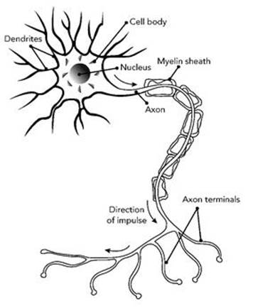
Fig 34 Nerve cell.

By connecting axons to dendrites, nerve cells can form structured networks. The mathematics of such networks, which we’ll get to in due course, shows that the resulting dynamics can be far more complicated than anything the component nerve cells can do on their own, just as a computer can do things that a transistor cannot. However, even a single nerve cell is a complicated thing to describe and model mathematically.

Scattered through the body are many different specialised networks of neurons, which cause muscles to contract or detect and process sensory data. Networks with just a few neurons can perform sophisticated tasks. Large networks of a few hundred are already too complex to understand in detail, and they can do many things that small networks can’t. A network of 100 billion neurons – a brain – poses a serious challenge for biologists and mathematicians alike. In fact, there is no real prospect of gaining a complete understanding: the brain is too complex. Nonetheless, a lot of progress is being made, because to some extent the brain has a modular structure, and we can study individual modules, which are simpler.

The simplest such module is a single nerve cell. If you can’t understand how a single nerve cell works, you won’t get far with an entire brain. One of the first significant applications of mathematics to biology occurred in neuroscience, the study of the nervous system, in 1952. The problem was the transmission of individual pulses of electricity along a nerve axon – the basis of the signals that are sent from one neuron to another. The Cambridge biophysicists Alan Hodgkin and Andrew Huxley developed a mathematical model for this process, now called the Hodgkin – Huxley equations.² Their model describes how an axon responds to an incoming signal received by the nerve cell. They were awarded a Nobel prize for this work.

Hodgkin and Huxley started from a physicist’s model of the nerve axon, treating it as a poorly insulated cable transmitting electricity. The insulation is poor because some of the atoms that take part in the associated chemical reactions can leak out. More precisely, what leaks is ions: charged atomic nuclei. The main vehicles of voltage leakage are sodium ions and potassium ions, but others, especially calcium, also play a role. So Hodgkin and Huxley wrote down the standard mathematical equation for electricity passing along a cable, and modified it to take account of three types of leakage: loss of sodium ions, potassium ions, and all other ions (mainly calcium). The Hodgkin – Huxley equations state that the electrical current in the cable is proportional to the rate of change of the voltage (this is Ohm’s law, a simple and basic piece of the physics of electricity), together with additional terms that account for the three types of leakage.³

The actual equations are messy, because of the complicated form of the leakage terms, and can’t be solved by a formula, so Hodgkin and Huxley did what all scientists and mathematicians do in such circumstances: they solved the equations numerically. That is, they calculated very good approximations to the solutions. There were already excellent, long-established methods for doing that, and yet another branch of mathematics, numerical analysis, entered the story. They did not have a computer; hardly anyone did in those days, and those that existed were the size of a small house. So they carried out the calculations by hand using a mechanical calculator. The result was that a voltage spike should travel along the axon (see Figure 35). With specific values for various data, derived from experiments, they calculated how fast the spike travelled. Their figure of 18.8 metres per second compared well with the observed value of 21.2 metres per second, and the calculated profile of the spike was in good agreement with experiment.

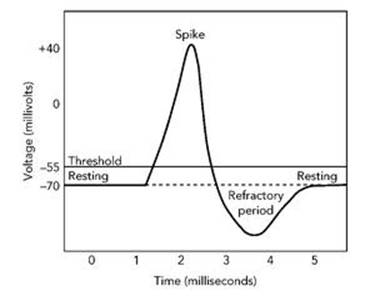
Fig 35 Voltage spike predicted by the Hodgkin – Huxley model.

The spike has some important features, which gave some insight into how a nerve cell works. The incoming signal has to be greater than a particular threshold value before the nerve cell fires and triggers a spike. This prevents spurious outgoing signals being triggered by low-level random noise. If the incoming signal is below the threshold, the voltage in the axon bumps up slightly but then dies away again. If it is above the threshold, the dynamics of the nerve cell causes the voltage to increase sharply, and it then dies down even more sharply; these two changes create the spike. There is then a short ‘refractory period’ during which time the nerve cell does not respond to any incoming signal. This keeps the spikes separate (and spiky). After that, the cell is back at rest and ready to respond to the next signal it receives.

Today there are many mathematical models of a single nerve cell or axon. Some sacrifice realism for simplicity, and are even simpler than the Hodgkin – Huxley equations; others aim at greater realism, which automatically makes them more complicated. As always, there is a trade-off: the more features of the real world you put into the model, the harder it becomes to work out what it can do. The goal, not always attainable, is to retain the features that matter and discard everything that’s irrelevant.

One of the simplest models yielded a valuable insight: the nerve axon is an excitable medium. It responds to a small input by amplifying it; then it temporarily switches off the amplification process, so that the resulting signal cuts off at some finite value instead of rising indefinitely. The model concerned derives from Richard Fitzhugh’s work at the National Institutes of Health at Bethesda in Maryland in the early 1960s, and is known as the FitzHugh – Nagumo equations.⁴ FitzHugh made conscious mathematical simplifications to the Hodgkin – Huxley equations, combining the roles of the ionic pathways into a single variable. The other key variable is the voltage. So the FitzHugh – Nagumo equations are a two-variable system, and we can represent those variables as the two coordinates of a plane. In short, we can draw pictures.

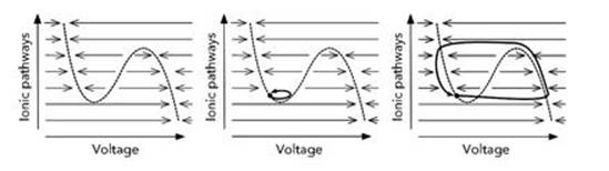
Fig 36 Excitability in the FitzHugh – Nagumo equations. Left: Direction in which the voltage changes. Middle: A small kick dies out and the state returns to rest (black dot). Right: A large kick triggers a voltage spike followed by a slow return to rest.

Figure 36 shows the most important feature of the FitzHugh – Nagumo equations: excitability. The left-hand picture shows a wiggly curve in the plane of the two state variables: this is the curve on which the voltage would not change as time passes if the ionic currents were fixed. The arrows show the direction in which the voltage changes as time passes. The middle picture shows the effect of a small disturbance, or ‘kick’, produced by an incoming signal. The state is disturbed from rest, but fails to cross the dotted curve, so it makes a small excursion and returns rapidly to its resting state. The right-hand picture shows the effect of a larger kick. Again the state is disturbed from rest, but now it crosses the dotted curve, so it makes a large excursion and eventually returns, slowly, to its resting state. This property is called excitability, and it is one of the central mathematical features of both the Hodgkin – Huxley and FitzHugh – Nagumo models. Excitability is what allows the neuron to generate a large voltage spike when given a small but not too small kick, and then return to rest reliably, even if a further signal comes in which might interfere with that process.

This sequence of events shows how a neuron obeying the FitzHugh – Nagumo equations can generate a single, isolated voltage spike. Real nerve cells do this, but they also generate long trains of pulses – they oscillate. Similar pictures reveal that the FitzHugh – Nagumo model can also produce oscillations.

This is just the simplest model for nerve cell dynamics. There are many others, and which is appropriate depends on the question being answered. The more powerful your computer, the more ‘realistic’ the equations can be made. But if the model gets too complicated, it often yields little insight beyond ‘it does so-and-so because the computer says so’. For some questions, a simpler but less realistic model may be better. This is the art of mathematical modelling, and it is more of an art than a science.

Excitability is one of the reasons why nerve cells can send one another signals. In fact, it is why signals can be produced to begin with. But the really interesting behaviour arises when several cells send signals to one another. Nerve cells in real animals form complex networks. Mathematical biologists are just beginning to grasp the amazing power of networks. A network of relatively simple components, communicating via little more than series of spikes, can do extraordinary things. In fact, they can probably do everything our brains can do, as far as manipulating sensory inputs and generating outputs to the body are concerned. This seems likely because the brain is a very, very complex network of nerve cells. And there are good reasons to think that most of the brain’s astonishing abilities are consequences of the network architecture.

One of the biological topics that I’ve worked on myself provides a nice example of networks of nerve cells. The topic is animal locomotion: how animals move using their legs, what patterns they use, and how those patterns are produced. This is a huge subject in its own right, with a fascinating history, but I can only scratch the surface here.

In July 1985, along with two other mathematicians and a physicist, I was travelling through redwood and sequoia forests down the coast of California in a Mini. We were on the way home from a mathematics conference in Arcata, a small town about 200 miles north of San Francisco. To pass the time when we weren’t hopping out of the car to look at giant trees, Marty Golubitsky (one of the mathematicians) and I started thinking about the patterns that form when you hook a lot of identical units together into a ring.

We’d already sorted out a general method for approaching this sort of question. It predicted that rings of this kind should generate travelling waves, in which successive units round the ring do exactly the same thing, but with a time delay. The simplest example is to hold your arms out sideways and let them dangle from the elbows. Now let the dangling bits swing to and fro. Typically, they either synchronise, with both arms moving in the same way, or they anti-synchronise, with the left arm doing the exact opposite of the right.

Similar patterns arise when there are more than two components. For instance, if you hook four components together in a square, with each one connected to the next, then you can get patterns in which all four components oscillate periodically, but there is a time difference of one-quarter of the period between each component and the next. It’s like four people all singing the same four-beat bar of music over and over again, but one starts with the first note, the next starts with the second note, the next with the third note and the last one with the fourth note.

Later, we realised that similar patterns occur in animal locomotion. Animals move in a variety of patterns, called gaits, repeating the same sequence of movements over and over again in a series of ‘gait cycles’. A horse, for example, can walk, trot, canter or gallop – four distinct gaits, each with its own characteristic pattern. In the walk, the legs move in turn, and each hits the ground at successive quarters of the gait cycle. So the sequence goes left back, left front, right back, right front, all equally spaced, over and over again. The trot is similar, but one diagonal pair of legs hits the ground first, and the other pair does so half a gait cycle later. So in both gaits all four legs do essentially the same thing, but with specific differences in the timing.

There are ten or twelve common patterns in animal gaits, and dozens of uncommon ones. Some animals, such as the horse, use several different gaits. Others use only one, other than standing still. Four of the most common gaits are illustrated in Figure 37.

Jim Collins, a biomechanicist (someone who applies mechanics to biology, especially medicine) at Boston University’s medical institute heard of our ideas, and he told us that gaits are thought to be produced by a relatively simple circuit in the animal’s nervous system, known as a central pattern generator (CPG). This is located not in the brain, but in the spine, and it sets the basic rhythms, the patterns, for the movement of the muscles that actually causes the animal to walk, trot, canter or gallop.

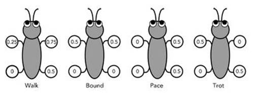
Fig 37 Some of the common four-legged gaits. The numbers show the fraction of the gait cycle at which each leg hits the ground.

No one had actually seen a CPG at this time. Their existence was inferred indirectly, and in some quarters they were a bit controversial, but the evidence was quite strong. However, the exact network of connections among the nerve cells was unknown. So we did the best we could and worked out the most plausible patterns, assuming various more or less natural structures for the CPG. We started with quadrupeds, and went on to apply similar ideas to sixlegged creatures: insects.

There had already been a lot of work done on the mechanics of legged locomotion. Our approach was more abstract, trying to infer the structure of a hypothetical CPG from the patterns observed in the legs. But it had an interesting consequence: it revealed that the same network of nerve cells, operating under different conditions, is capable of generating all the most symmetric quadruped gaits – and, in more subtle circumstances, less symmetric ones like the canter and the gallop as well.

None of the networks that we proposed was completely satisfactory, for various technical reasons. Discussions with Golubitsky and the Ontario-based mathematician Luciano Buono led to the insight that any workable CPG for quadrupeds must have at least two units per leg: one to work the muscles that flex the leg and the other to work the muscles that extend it. So the most natural CPG for quadrupeds should have eight units (Figure 38, see over).⁵

This network can generate all the basic four-legged gaits. Along with the standard gait patterns, it predicted one that we’d not encountered before. In this gait, which we named the jump, the two rear legs hit the ground together, and then the two front legs hit the ground together a quarter of the way through the gait cycle. If it had been halfway through the cycle, this gait would have been a standard one, the bound. Dogs bound when running fast, for example. But one-quarter of the way through the gait cycle was a real puzzle, especially since no legs hit the ground halfway through or three-quarters of the way through. It was as though the animal were somehow suspended in mid-air.

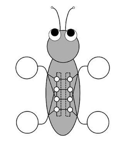
Fig 38 Predicted architecture of quadruped CPG. Two rings of four identical modules are linked left – right. Two modules connect to each leg, determining the timing of two muscle groups. The picture is schematic and there may be many more connections in the CPG, but having the same symmetry.

We came to this conclusion late one afternoon. The Houston Livestock Show and Rodeo was in town, and we had seats booked for that evening. So we went to the Astrodome, and watched cattle being roped and buggies being raced. Then came the bucking broncos. The horses were trying to throw the riders off their backs, and the riders were trying to stay on for as long as they could – which was often just a few seconds. Suddenly Golubitsky and I looked at each other and started counting ... The horse that we were watching was jumping into the air, both back feet giving it a push, then both front, then hanging in the air ...

It looked very much as though the difference in timing was one-quarter of the full gait cycle. The Exxon Replay, a television recording in slow motion, of that precise horse confirmed this. We had found our missing gait.

Later we discovered that two other animals, the rat and the Asia Minor gerbil, also employ this unusual gait. We found several other features of real gaits that were predicted by our eight-unit CPG or natural generalisations, including one displayed by centipedes. Of course none of this proved that our theory was correct, but it did mean that it passed several tests that might prove it wrong.

More recently, Golubitsky and the Portuguese mathematician Carla Pinto have applied the same idea to a four-unit network for biped gaits – two legs, like us.⁶ They find ten gait patterns, eight of which correspond to known gaits in bipeds. They include the walk, run, hop and skip.

Another fascinating network of neurons is definitely found in a real animal, rather than being a mathematician’s pipe-dream. It is the CPG for the heartbeat of the medicinal leech Hirudo medicinalis.

Leeches are slug-like creatures that suck blood. They were widely used in ancient medicine to ‘balance the body’s humours’ when there was deemed to be an excess of blood; the earliest record of their use goes back to 200 BC. The use of leeches died out during the nineteenth century, but by the beginning of the twenty-first they were back in vogue, though for more scientific reasons and in a more limited realm. The saliva of leeches contains a molecule called hirudin, which keeps blood flowing freely while the animal sucks it from its victim. Hirudin helps to stop the patient’s blood coagulating during microsurgery.

The medicinal leech poses a curious problem for mathematicians interested in networks of neurons: its heartbeat follows a very strange pattern. The heart of a leech consists of two rows of chambers, with about 10 to 15 in each row, depending on the species. The pattern goes like this. For a while, all the chambers on the left beat in synchrony – at the same moment. While this is happening, the chambers on the right beat in sequence, one after the other, from back to front. After between 20 and 40 beats, the two sides swap roles. Then they swap again, and so on.

Nobody really knows why the leech heart beats in this manner, but the blood pressure is high when the chambers beat in sequence, and much lower when they beat synchronously, so the need to avoid persistent high pressure (or indeed persistent low pressure) may be part of the reason. We have a much more complete explanation of how it does it. The strange switching between two patterns is driven by the creature’s nervous system, and is a natural feature of network dynamics (Figure 39, see over).

Ronald Calabrese and colleagues at Emory University in Atlanta, Georgia have investigated the heartbeat of the leech in an extensive series of papers.⁷ They traced the dynamics to a CPG: a network of nerve cells located in most of the leech’s 21 segments. In each segment there is a pair of motor neurons, one on the left and the other on the right, which make the heart muscles contract (see Figure 40). There is also a pair of ‘interneurons’, which help to generate the pattern of nerve impulses needed to control the heartbeat. The interneurons in the third and fourth segments are wired up to produce a regularly pulsing timing pattern; in effect they form a clock whose regular ticking influences what the other neurons do. The wiring in the fifth, sixth and seventh segments directs these signals to the heart motor neurons on left and right sides of the leech, and modifies the signals so that on one side the effect is a sequential wave of contractions, but on the other all muscles contract simultaneously. The dynamics of these three segments switches regularly from this pattern to its mirror image.

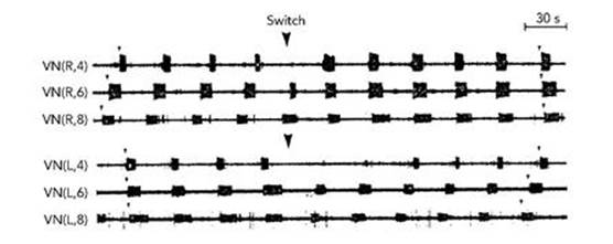
Fig 39 Recordings from various vascular nerves of a leech reveal short bursts of electrical activity. Here the 4th, 6th and 8th nerve cells on the right side of the leech (the top three rows of signals) are bursting in sequence before the time marked with an arrow, but in synchrony after that. The corresponding nerve cells on the left side of the leech (the bottom three rows) initially burst in synchrony, but switch to bursting in sequence.

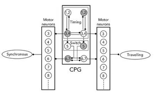
Fig 40 CPG for the leech heartbeat.

Calabrese’s group originally focused mainly on these timing circuits, and did not investigate in any detail how the timing signals are transmitted to segments further along the leech. In 2004 Buono and Antonio Palacios, of the Nonlinear Dynamical Systems Group at San Diego State University, employed techniques from dynamical systems with symmetry to model this transmission process.⁸ They modelled the network that transmits the signals as a chain of neurons whose ends are linked to form a closed loop. Symmetric dynamics tells us that there are two common patterns of periodic oscillation in closed loops: sequential and synchronous. The relations between the two patterns arise through a so-called mode interaction, when the parameters of the network connections cause both patterns to arise simultaneously.

In earlier work by Buono and Golubitsky, mode interactions of this type were invoked to explain the less-symmetric gaits of quadrupeds, such as the canter and gallop of a horse. So the cantering horse and the heartbeat of the leech fall into the same category of phenomena, both mathematically and biologically.

More recently, Calabrese’s group has devised more detailed models, with an emphasis on the structure of the signals between nerve cells, which occur in short bursts (as shown in Figure 39). The role of bursting seems to be central to this and many similar problems in neuroscience, so mathematicians have developed equations for bursting neurons.

Networks of neurons are involved in perception as well as motion.

In 1913 the New York neurologists Alwyn Knauer and William Maloney published a report in the Journal of Nervous and Mental Disease on the effects of the drug mescaline, a psychedelic alkaloid found in cacti, notably peyote, which grows in desert areas of Central America. Their subjects reported striking visual hallucinations:

Immediately before my open eyes are a vast number of rings, apparently made of extremely fine steel wire, all constantly rotating in the direction of the hands of a clock; these circles are concentrically arranged, the innermost being infinitely small, almost point-like, the outermost being about a meter and a half in diameter. The spaces between the wires seem brighter than the wires themselves ... The center seems to recede into the depth of the room, leaving the periphery stationary, till the whole assumes the form of a deep tunnel of wire rings ... The wires are now flattening into bands or ribbons, with a suggestion of transverse striation, and colored a gorgeous ultramarine blue, which passes in places into an intense sea green. These bands move rhythmically, in a wavy upward direction, suggesting a slow endless procession of small mosaics, ascending the wall in single files ... Now in a moment, high above me, is a dome of the most beautiful mosaics ... Circles are now developing upon it; the circles are becoming sharp and elongated ... now all sorts of curious angles are forming, and mathematical figures are chasing each other wildly across the roof.

Similar effects can be seen by closing your eyes and pressing on the eyeballs with your thumbs, so a first guess might be that the drug affects the eyes. Actually, it affects the brain, creating signals that the brain’s visual system interprets as images seen by the eye (see Figure 41). These patterns offer important insights into the structure of the visual system, thanks to a mixture of experiments and mathematical analysis.

A large part of the brain is devoted to the visual system. Biologists have been studying the neuroscience of vision for many years, and have learned a lot about it. But there’s a lot that we still don’t understand. At first sight, you may wonder what the problem is. Isn’t the eye basically a camera – a pinhole camera with the pupil as a pinhole, a lens to improve the focus and a retina to receive the image? The main problem is that the brain doesn’t just passively ‘take a photograph’ of what is out there. It provides automatic understanding of what the eye is seeing. The brain’s visual system processes the image, working out what objects are being viewed, where they are relative to one another, even decorating them with the vivid colours that we perceive. We look out of the window and instantly ‘see’ a man walking past with his dog. But the dog is passing behind a lamppost, and half the man is hidden from view by a hedge; the man’s body is mostly covered by a coat and his face is obscured by the hood. Moreover, the image appears to be three-dimensional: we know, without thinking, which parts are in front of which.

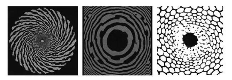
Fig 41 Hallucination patterns. Left: Spiral. Middle: Tunnel. Right: Honeycomb.

It has proved almost impossible to teach a computer to analyse such a scene and recognise the main objects in it, let alone work out what they are doing. Yet the visual system achieves this, and more, in real time, with a moving image. With the help of some clever biochemistry and difficult experiments, mathematical biologists are starting to make inroads into the structure and function of the visual system. And what we currently understand shows that evolution has been very clever indeed.

Images received by the retina of each eye pass along the corresponding optic nerve (actually a huge bundle of nerve fibres) to an area of the brain known as the visual cortex. This lies on the surface of the brain, just under the skull, and if you were to lift off the top of the skull you would see that it has the familiar convoluted shape, a bit like a cauliflower. If you flatten out the convolutions, the visual cortex turns out to be made from a number of layers of nerve cells, placed on top of one another. The top layer, known as V1, starts by representing the image as an array of on/off signals in the corresponding nerve cells. In experiments, it proved possible to work out what a cat was looking at by using voltagesensitive dyes to make the on/off pattern visible. If the cat was looking at a square, say, then a distorted square appeared on the V1 layer.

Each layer of the cortex is connected to those above and below, and this wiring is done in such a way that successive layers extract different information from the basic image formed on the top layer. The next layer down, for example, sorts out the boundaries between different features of the image – where, say, the dog’s body appears to be cut by the edges of the lamppost, and where the man’s hood ends and the house behind it begins. It also works out the orientations of these boundaries. Then the next layer can compare directions and locate such things as the dog’s eyes, which are point-like, so the edges change direction very rapidly. Presumably, many layers down, is a nerve cell or a network of them that makes the deduction ‘dog’; after that comes the recognition that the dog is a Labrador retriever, until at some level you realise that it’s Mr Brown taking Bonzo for his evening walk.

There are useful mathematical models of the first few stages of this process, which have a very geometric feel to them. These models show how information flows back up through the layers as well as down into the depths, priming the visual system actively to look for specific features. This is how our eyes track the dog as parts of it vanish behind the lamppost and reappear. It ‘knows’ that they are going to do that, and anticipates it. It is possible to devise experiments that make use of the visual system’s ability to anticipate what it expects to see, by tricking it into seeing something else. It is also possible to alter the brain’s perceptions using drugs. Recent discoveries about the V1 layer of the visual cortex depend, to some extent, on the patterns that arise when volunteers take hallucinatory drugs such as LSD.

Legal experimental volunteers and illicit users of these drugs report seeing a variety of strange, geometric patterns. It can be shown that the patterns do not originate in the eye, even though they are ‘seen’ to be part of the image that the eye is receiving. Instead, they are artefacts caused by changes in the way the nerve cells in the cortex function. Anything that the brain’s networks perceive is automatically interpreted as though it had come from an external image. We can’t stop that happening; it is how we see everything. What we fondly imagine to be the external world is actually a representation held in our own heads. This is the main reason why the visual system can be tricked into seeing things that aren’t there. On the whole, though, we can trust our visual system, which evolved to perceive things that are there. Except when it is presented with carefully contrived images that create illusions, or drugs that cause hallucinations.

Around 1970, Jack Cowan, a biomathematician now at Chicago, started to use hallucination patterns to unravel the structure of V1. His first discovery provided strong evidence that hallucination patterns arise in the brain, not the eye. The range of reported hallucination patterns is huge, but most of them are variations on a basic theme: spirals. Some are concentric circles, and a circle is what happens to a spiral when it is wound so tightly that the spacing between successive turns becomes zero. Others are radial spokes, another special case when the turns of the spiral grow so rapidly that the spacing effectively becomes infinite. Sometimes the spiral pattern is decorated with hexagons, like a honeycomb; sometimes it is covered in a chequered pattern of lozenges, like Elizabethan window panes. Sometimes it is too bizarre to describe meaningfully. But spirals dominate, and they are of the type that mathematicians call logarithmic. Spirals and spokes often rotate, and concentric circles can spread like the ripples on a pond when you drop a stone into it.

To form a logarithmic spiral, imagine a spoke that rotates at constant speed, and a point that moves outwards along the spoke. The combination of these two motions creates a spiral, but the exact shape of the spiral depends on how the point moves along the spoke. For example, if it travels at a fixed speed, we get an Archimedean spiral, in which successive turns are equally spaced. If the speed grows exponentially, so that (say) each turn is twice as far out as the previous one, we get a logarithmic spiral (see Figure 42).

In 1972, Cowan and his collaborator Hugh Wilson wrote down mathematical equations, now called the Wilson – Cowan equations, which describe how a large number of interconnected neurons interact with one another.⁹ In 1979 Cowan and Bard Ermentrout used these equations to model how waves in the visual cortex propagate, and deduced that the complex spiral patterns reported by experimental subjects can be explained in terms of much simpler patterns of electrical and chemical activity in the top layer of the cortex. The predominantly spiral nature of the hallucinations is a useful clue, because physiologists have figured out how the image sent to the cortex by the retina compares to the one that the cortex actually receives. The retina is circular, but the V1 layer, when unfolded, is roughly rectangular. The image on the cortex is a distorted version of the image on the retina. The way it is distorted can be described by a mathematical formula which has the effect of converting radial lines on the retina into parallel lines on the cortex, and concentric circles on the retina into another set of parallel lines, at right angles to the first. However, just to keep us on our toes, this happens in two different regions of the cortex. In reality they are joined like an hourglass, as in Figure 44, but mathematically it is often convenient to swap the two ends to make an oval shape, as in Figure 43.

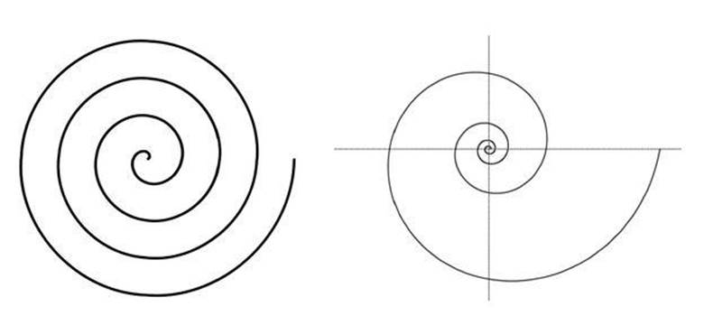
Fig 42 Left: Archimedean spiral. Right: Logarithmic spiral.

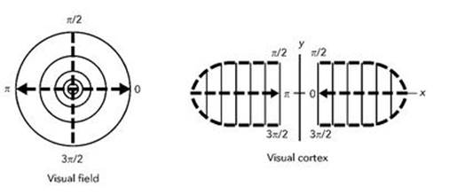
Fig 43 Retino-cortical map.

The most significant feature of this ‘retino-cortical map’ is that it turns logarithmic spirals on the retina into parallel lines in the cortex. The visual system automatically makes us ‘see’ anything detected by the cortex, whether or not it originates in the eye, so we will ‘see’ spirals if something creates a pattern of parallel stripes on the cortex. Psychotropic drugs cause waves of electrical activity, and the simplest wave pattern is stripes.

If the stripes move, forming travelling waves like ocean waves coming up a beach, then the geometry of the retino-cortical map implies that the spirals will appear to rotate. Radial spokes are a special case of spirals, and correspond to horizontal stripes on the cortex (relative to the conventional orientation of the cortex). As the waves travel across the cortex, the spokes rotate. Concentric circles similarly correspond to vertical stripes; this time, as the waves travel across the cortex, the circles appear to expand from their centre (see Figure 44).

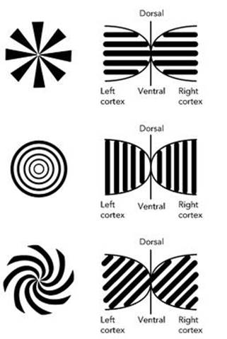
Fig 44 Hallucination patterns and the corresponding waves in the cortex.

This already offers a big clue about the hallucination patterns: they make much more sense if they are caused by simple striped waves, moving across the cortex. And those waves are patterns of electrical and chemical activity, caused by the drug. The other more elaborate patterns sometimes reported have a similar explanation, involving different behaviour on the cortex. The spiral honeycombs, for instance, correspond to straightforward honeycomb patterns on the cortex.

The equations that Cowan and Ermentrout devised constitute what mathematicians call a continuum model. That is, it models the very fine but discrete network of real neurons by a continuous distribution of infinitesimal neurons. The cortex becomes a plane, and the neurons reduce to points. This kind of transition from discrete reality to a continuous model has become a standard strategy when applying mathematics to the real world, because it permits the application of differential equations, a very powerful tool. Historically, the first areas of science to be treated this way were the movement of fluids, the transfer of heat and the bending of elastic materials. In all three cases, the real system is composed of discrete atoms, which though very small are indivisible, whereas the mathematical model is infinitely divisible. Experience shows that continuum models are very effective provided the discrete components are much bigger than the effects being described. Although neurons are much larger than atoms, they are considerably smaller than the wavelengths of electrical waves in the cortex, so it is reasonable to hope that a continuum model might be worth pursuing.

A further simplification replaces the oval shape of the flattenedout cortex by an infinite plane. The modelling assumption here is that the edges of the cortex do not have a significant effect on waves in its interior. With all these simplifying assumptions in place, standard methods used to study pattern formation can be applied to classify the wave patterns in the cortex, and hence the hallucination patterns.

Initial attempts to analyse travelling waves in the cortex using these methods scored some successes, but didn’t always get the details right. When new experimental methods revealed the ‘wiring diagram’ for neurons in the cortex, it became clear why this was happening, and suggested a slightly different model.

Cells in V1 do not just map out the image, like a collection of pixels on a TV screen. They also sense the directions of edges in the image. So the state of a cell is not just the brightness of the corresponding point in the image (I’m ignoring colour here and thinking about just one eye) but also the local orientation of any lines in the image. Mathematically, each point in the plane has to be replaced by a circle of orientations. The resulting shape does not correspond naturally to a shape in our familiar three-dimensional space, but we don’t need to visualise it in order to do the sums.

Experiments show that the neurons in V1 are arranged in small patches, and within each patch the neurons are especially sensitive to a particular orientation. Neighbouring patches respond to nearby orientations, so that (say) one patch might respond to vertical edges, and a neighbouring patch might respond to edges tilted 30° to the right of vertical. Most of the connections among these neurons fall into two types. Within any given patch, we find shortrange inhibitory connections, meaning that incoming signals suppress activity in the nerve cell instead of stimulating it. But there are also long-range excitatory connections between distinct patches, and they do stimulate activity. Moreover, the excitatory connections are aligned along a specific direction in the cortex: the same direction that the patch itself prefers.

This pattern of connections changes the corresponding continuum model, which is not a plane’s worth of points, but a plane’s worth of circles. Translations and reflections behave in the usual way. However, any rotation of the plane must also rotate every circle, otherwise the wiring diagram doesn’t work out properly. Once the experiments have shown how to puzzle out the correct model, the heavy machinery of the mathematics of pattern formation can be brought to bear.¹⁰ This time, the classification of the wave patterns in the cortex, and the corresponding hallucinations, performs better.

The new mathematical model provides a convincing catalogue of hallucination patterns, and it also suggests the reason for the wiring diagram that nature has evolved for the V1 layer of the cortex. Imagine one of the patches, and suppose that it ‘sees’ a short segment of horizontal line. Its local inhibitory connections effectively vote for the most plausible direction for this line: the direction that receives the strongest signal wins, and all other orientations are suppressed. But now that patch sends excitatory signals to patches that are sensitive to that same orientation, in effect biasing them in favour of the same orientation. And it sends this signal only to patches that lie along the continuation of the direction that it has selected. The net result is that the direction of the line, as seen by this patch, is tentatively extended across the cortex. If this extension is correct, the next patch across will reinforce that choice of direction. However, if the next patch detects a strong signal in a different direction, then this will override the bias signal that is attempting to extend the edge.

In short, the nerve cells are wired so that they fit local bits of edge together into longer lines in the most plausible fashion. Any small gaps in these lines will be ‘filled in’ by the excitatory signals; however, if the line changes direction, the local inhibitory signals will confirm that this has happened and settle on a new choice. So the end result is that V1 creates a series of contours – linear outlines of the main features in the image. In 2000, John Zweck, a mathematician at the University of Maryland, and Lance Williams, a computer scientist at the University of New Mexico, used exactly the same mathematical trick to devise an effective algorithm for their work on computer vision.¹¹ The application was contour completion – filling in missing bits of edges in an image, for example where part of one object is hidden behind another.

Like the dog partly hidden by the lamppost.

Neuroscience is one of the most active areas of mathematical biology. Researchers are working on a huge variety of topics: how neurons work, how they link up during development, how the brain learns, how memory works, how incoming information from the senses is interpreted. Even the more elusive aspects of the human brain, such as its relation to mind, consciousness and free will, are also under investigation. The techniques employed include dynamics, networks and statistics.

In parallel with these theoretical developments, biologists have made major advances in experimental techniques to study what the brain is doing. There are now several ways to image the activity of the brain in real time – in effect, to watch which parts of the brain are active, and how the activity passes from one region to another. But the brain is immensely complex, and at the moment it is probably better to focus on specific features of the nervous system, rather than trying to understand the whole thing in one go. Our brains are so complicated that, ironically, they may be inadequate to understand ... our brains.