Mathematics of Life (2011)
Chapter 12. Knots and Folds
The discovery of the genetic code, which represents amino acids in proteins as triples of DNA bases, was the first of many breakthroughs where DNA was thought of as a code, a list of symbols. But the physical form of the DNA molecule is also important, and so are the forms of the molecules that it encodes.
The same goes for proteins. To make an organism, you need more than a list of proteins: you need to get the right proteins into the right places at the right time. Just as you can’t make a cake by dumping all the ingredients into a bowl and sticking it in the oven, you can’t make an organism by making 100,000 proteins and hoping that they will somehow sort themselves out into an amoeba or a human being.
Only a small proportion of the genome consists of genes – codes for proteins. For a long time the rest was stigmatised as ‘junk DNA’, evolutionary relics with no current function, going along for the ride because it wasn’t worth evolution’s while to weed them out. It is now clear that at least some of that junk DNA helps to control how an organism is assembled. The rest may still be junk – but I wouldn’t bet on it, given the past record.
How does this DNA control system work? The answer might require no more than the cracking of some other code, the code for instructions rather than ingredients. But again it’s not that simple. One of the systems that control an organism’s development uses genes (more properly, the proteins they encode) to switch other genes on and off. What matters here is the dynamics of the genetic switching network. And dynamics is a matter for mathematics, it can’t just be read off from DNA codes. You might, perhaps, be able to read off which genes act on which other ones – but that information won’t tell you what they all do when everything is happening at once. In the same way, knowing how temperature and humidity in the Earth’s atmosphere affect each other doesn’t tell you next week’s weather.
The shapes of the molecules turn out to be at least as important as the sequences that determine them. The double-helix shape of DNA governs many of its most basic properties. In particular, the copying system for DNA, which cells and indeed the entire organism use to reproduce, must overcome a massive topological obstacle: the two DNA strands are twisted round each other like the strands of a rope. If you try to pull a rope apart by tugging on its strands, all you get is a hopeless tangle.
The shape of a protein is more important still. Many proteins do their jobs by binding to other proteins – sticking to them, usually temporarily, but in a controllable way. When the protein haemoglobin picks up or releases a molecule of oxygen, it changes shape. A protein is a long chain of amino acids, and it gets its shape by folding up into a compact tangle. In principle, the shape of this tangle is determined by the sequence of amino acids; in practice, it’s virtually impossible to calculate the shape from the sequence. The same sequence can fold up in a gigantic number of ways, and it is generally thought that the actual shape it chooses is the one with the least energy. Finding this minimal energy shape, among the truly gigantic list of possibilities, is a bit like trying to rearrange some list of thousands of letters of the alphabet in the hope of getting a paragraph from Shakespeare. Running through all the possibilities in turn is totally impractical: the lifetime of the universe is too short.
One of the keys to the mysteries of DNA shape is a branch of mathematics known as topology. As a well-developed area, topology has been around for little more than a century, though with hindsight a few precursors can be detected. By the 1950s it had shot to stardom, becoming one of the central pillars of pure mathematics, but its role in applications was still relatively minor. It clarified some theoretical issues in the dynamics of the Solar System, for instance. Topology is important in pure mathematics because it provides conceptual machinery to deal with any question involving continuity. And continuity – transforming shapes and structures without tearing them apart or breaking them into separate pieces – is a common theme in many different areas of mathematics. It is a common theme in applications, too: most physical processes are continuous. But it’s not straightforward to deduce anything useful from that property, and it took a lot longer for topology to find a role in applied science.
Topology is not included in school mathematics lessons, except for a few cute but inconclusive tricks. A typical example is the Möbius band, invented independently by August Möbius and Johann Listing in 1858. Take a long strip of paper, bend it round to bring the ends together like a dog collar, twist one end through half a turn, and then glue the ends together. The resulting surface has several counter-intuitive properties: it has only one side, and only one edge, and if you cut it along the middle it does not fall apart into two separate pieces. There are a couple of practical applications of Möbius bands: conveyor belts that last twice as long before they wear out, and a method for connecting electrical wiring to a rotating object. But none of that is terribly impressive.
There is a lot more to topology, but the concepts are too abstract to be explained easily or accurately without a lot of technical background. However, the pure mathematicians’ nose for an important idea has eventually been vindicated, and topological methods are being used in an increasingly broad range of real-world problems, from biology to quantum field theory. The application that I will describe here has yielded some crucial insights into the workings of DNA. The topological gadgetry that comes into play is less technical than in most other areas of applied maths – and is something we all come across almost every day.
Knots.
Knots tend to be associated with tying parcels, boy scouts, sailing and mountaineering. Centuries of trial and error have shaped our understanding of knots: which one to use in which circumstances. Tie a pig to a square post with a clove hitch and you’re in trouble; if the pig runs round the post in the right direction, the knot obligingly unties, and off goes your bacon.
The topology of knots tackles two general questions. One is to decide whether two knots are topologically the same, that is, whether each can be changed into the other by a continuous transformation. If you tie one of them in a length of string, can you twist the string to get the other knot? A special case of this question is to determine when an apparently complicated knot is really unknotted (see Figure 45). The second topological question is much more ambitious: whether we can classify all possible knots. There are infinitely many knots, and even the simpler ones, with few crossings, provide a rich variety of types.
Any knot tied in a length of string can be untied by reversing the process; then you can retie the string into any other knot that you wish. To get a sensible question, we have to do something to stop the knot escaping off the end of the string. The time-honoured solution in topology is to glue the ends of the string into a closed loop. So a topologist’s knot is a knotted circle, rather than a knotted curve with ends. For instance, the two knots in Figure 45 then look like Figure 46.
We can now rephrase the question in the caption to Figure 45 in knot-theoretic terms. One of the two ‘knots’ below is actually unknotted: you can transform it, continuously, into a perfect circle, with no crossings. The other is a genuine knot, and can’t be untied without cutting the string. So the question is, which is the knot, and which the unknot? In fact, the more complicated-looking knot, on the right, is the one that unties. The other is a reef knot, and generations of boy scouts know that it does not untie. But that’s not a mathematical proof, and what boy scouts mean by ‘untie’ includes things like free ends and the possibility of the knot slipping. So topologists have to be more careful, and find solid logical proofs for things that seem obvious.
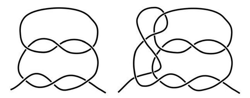
Fig 45 Pull on the ends – which one unknots?
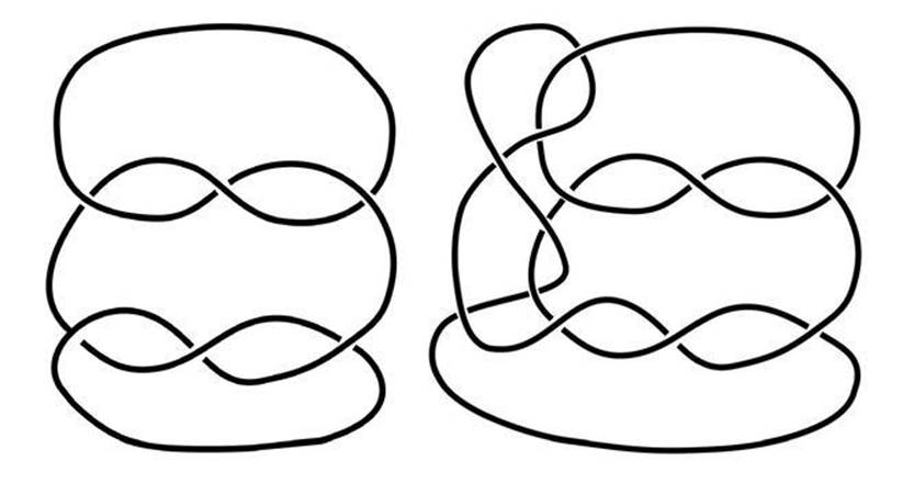
Fig 46 Glue the ends to stop the knot escaping.
Knot theory has on occasion been ridiculed as pseudointellectual trivia. That’s an understandable attitude if you don’t know any mathematics and base your opinion on the everyday meaning of the word ‘knot’, but when it comes to mathematical concepts that’s a rather silly way to think. It’s like expecting quantum field theory to be solely about sheep. The mathematics of knots has turned out to be deep and difficult, and it has been a prime mover in the development of topology.
Knot theory is useful in biology because DNA ties itself in knots. The knots are a relic of the twisted topology of the double helix. If you cut a length of DNA and join its ends together, two things can happen. Either you have joined each separate helix to itself, in which case you end up with two closed loops of single-strand DNA. Usually, these are linked to each other – impossible to separate without cutting. Or, you must have joined each strand to the other one. Now they form a single closed loop, and typically it is knotted.
If you can understand these knots and links, you can work out features of the biological process that did the cutting. And this is an important idea, because nature has to cut and rejoin DNA on a routine basis. The complex topology of the double helix forces this. Copying a DNA strand requires cutting it, disentangling it from its partner, building the new copy, then putting the cut strand back where it came from and rejoining it (see Figure 17 on p. 98). These processes are very complicated on a molecular level, but they make life possible. And since they are on a molecular level, it’s not easy to observe them as they happen. Instead, they have to be inferred.
The method used to derive the double-helix structure of DNA is of little use here. It involves making a DNA crystal, illuminating it with X-rays and observing the resulting diffraction patterns. But cellular DNA is not a crystal. It is a free-moving molecule dissolved in a liquid. A new approach is needed to understand what DNA does in a cell.
The cellular machinery is not just the puzzle here: it also provides part of the answer. DNA is cut into pieces by special proteins, enzymes, known as topoisomerases. One way to find out what happens is to image the resulting strands using a very powerful electron microscope. Making these images required a new technique: coating the DNA strands with a special protein to make them thicker. The topology of those strands tells you useful things about the action of the topoisomerases. This in turn tells you things about the DNA. So you can get information about how topoisomerases do their work, and the effect they have on the DNA, by letting them cut up some DNA and seeing what shapes you get.
Biologists have discovered an effective way to keep this kind of investigation under control: perform the cutting operation on a closed loop of DNA, which can be constructed using standard techniques of genetic engineering and equipped with special regions whose code sequence can be recognised, and operated on, by a suitable enzyme. The result is either a DNA knot or two DNA loops that are linked together. The way the separate strands overlap can be observed with an electron microscope. Now you have a problem: you have a picture of a knot (similar to Figure 47), or a link – but which one is it? It may well be twisted and twirled in a way that makes the answer far from obvious. But topology can come to your rescue.
Knots are familiar, and seem simple, which suggests that they should be easy to understand. However, a quick glance at a book like the famous Ashley Book of Knots reveals the existence of thousands of different knots, and those are just the ones that turned out to be useful in the days of sailing ships, or are decorative, or can be used for party tricks. Distinguishing knots, and working out what happens to them when you make various types of change, are basic issues in topology. And they’re hard.
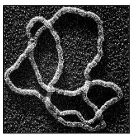
Fig 47 Twisted strands of DNA forming a Whitehead link.
For instance, although experiment made it clear thousands of years ago that a knotted length of string is different from an unknotted one, a solid logical proof of the existence of knots had to wait until the 1920s. The first big success of topological knot theory was a rigorous proof that the standard overhand knot, embedded in such a manner in a closed loop of string, cannot be untied. That is, no continuous transformation will convert it into an ordinary circular loop.
Why is this problem so difficult? It requires a proof that no transformation, however complicated and cunning, can do the job. It is much easier to analyse some specific transformation and see what it does, but this question can’t be answered that way. In principle, you have to contemplate all possible transformations, and show that none of them unties the knot. In practice this is impossible, but there is a clever way to achieve the same result without considering infinitely many, ever more complicated transformations. The idea is to look for an invariant – a specific quantity or structure associated with any knot that stays the same when the knot is transformed. The invariant must also be something we can calculate, otherwise it will be pretty but useless.
Here’s how an invariant does its job. Suppose, for example, that some cunning topologist invents an invariant, and when we calculate it, the answer is 3 for the overhand knot but 0 for the ‘unknot’, an unknotted loop. Then we can prove, with complete logical rigour, that no amount of twisting and turning and bending and stretching can convert an overhand knot into an unknot. Why? Because such transformations will always produce a knot whose invariant is 3. Since the unknot is not one of those, it can never be produced.
This is a straightforward and widely used idea, but there is a sting in the tail. First, the thing we’re thinking of does actually have to be an invariant, and it may not be easy to find such a beast – or to prove its invariance. Second, it must be something we can calculate for the knot we start from, and for the one we hope to finish with; here, the unknot. Third, it must be different for the initial knot and the final one.
Despite these obstacles, topologists managed to invent some decent knot invariants, and they used them to solve basic problems. Prove the overhand knot is genuinely knotted. Prove that you can’t transform an overhand knot into its mirror image. Prove that a reef knot is different from a granny knot, and both differ from the overhand knot. And so on.
Many of the more recent knot invariants are algebraic formulas, often called polynomials. There is a classic invariant of this kind, named for its inventor, James Waddell Alexander. You can calculate the Alexander polynomial from a picture of the knot. It is x-1-1+x for the overhand knot, and -x-1+3-x for the figure-of-eight knot. Since these are visibly different, so are the knots.
The Alexander polynomial solves some problems, but not others. It fails to distinguish reef from granny, and it can’t tell the difference between an overhand knot and its mirror image. So topologists sought improved invariants. Ideally, what we want is an invariant that completely distinguishes all topologically different knots: if the knots differ topologically, then their invariants have to be different too. But that proved elusive. However, Vaughan Jones invented a pretty good new invariant in 1983. The Jones polynomial can distinguish reef from granny, and tell the difference between an overhand knot and its mirror image. Other mathematicians generalised his ideas, and we now have several powerful knot invariants.
Invariants are not the only way to approach questions about knots. An earlier idea was to construct knots from simpler building-blocks, and try to understand how the blocks worked and how they fitted together. This technique is useful in understanding the action of enzymes. John Horton Conway, a British mathematician famous for his unorthodoxy, imagination and playful approach to much of mathematics, invented one such structure, known as a tangle.By this term, he meant a piece of a knot whose ends are attached to a surrounding box. You can transform the bits of knot in any continuous manner, as long as they remain inside the box, but you have to leave their ends attached to the surface. The basic type of tangle consists of two separate strands, each with two ends, so there are four ends on the box, and the strands themselves are knotted and linked together in the interior of the box. In Figure 48 the boxes are shown as squares, but they are really three-dimensional.
There is a trivial tangle, in which the two strands are parallel and do not link or twist. Tangles can be combined by ‘adding’ two of them together. To do this, sit them side by side, join adjacent ends, and replace the two surrounding boxes by a single, larger box. This is the sense in which tangles are building-blocks, and by repeated additions, finally joining corresponding free ends to close the loop, you can make knots from them. The trivial tangle acts like zero: adding it to another tangle just extends one pair of strands, and has no topological effect.
In 1985 Nicholas Cozzarelli, a molecular and cell biologist at the University of California at Berkeley, and colleagues, applied tangles to a problem about DNA called site-specific recombination.1 A site, in this context, is a short, two-stranded segment of DNA whose base sequence can be recognised by an enzyme. Two such sites can be recombined: the enzyme snips out corresponding segments of the two DNA chains that lie between them, swaps their ends round in some manner, and rejoins everything. Except for the business of surrounding boxes, this type of recombination has the same geometric effect as adding a new tangle to what was previously the trivial tangle.
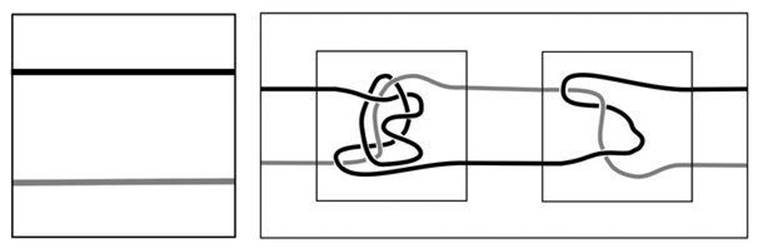
Fig 48 Left: trivial tangle. Right: Two tangles (inside small squares) and how to add them (outer rectangle). The shading distinguishes separate strands and has no other significance.
Thus armed, we can attack a genuine biological problem: the action of an enzyme with the impressive name Tn3 resolvase. This is a site-specific recombinase. A recombinase is an enzyme that breaks DNA strands and joins them together again in a different way; it is site-specific if the place where it makes these changes corresponds to a specific short DNA sequence. Tn3 resolvase can undergo several successive reactions of this kind with doublestranded DNA, and the problem is to find out exactly how the strands are broken and rejoined. The topological clues, which at first sight are rather puzzling, make it possible to reconstruct how the enzyme acts.
Begin with a circular loop of two-stranded DNA, which topologically is the unknot. Allow the enzyme to act on it once, and the result is the so-called Hopf link. About once in 20 times there is a second reaction, leading to the figure-of-eight knot. Much rarer, but possible, is a triple reaction, which gives the so-called Whitehead link (see Figure 49).
The single-step reaction is illustrated in Figure 50. The unknotted loop of DNA is twisted up so that it divides naturally into three regions, each of which constitutes a tangle. These regions are the parallel strands inside the enzyme (shaded circle), the double-twist to its left and the rest of the DNA. The one that most concerns us here is the first of these, which is where the enzyme rearranges the DNA strands, in a manner that is shown schematically in Figure 50 as a crossing-over of the two strands. But that’s just one guess at how the enzyme acts, and there are many other possibilities. The problem is to replace this schematic picture by the one that actually occurs in nature, just by looking at the range of knots and links produced by the chemical reaction.
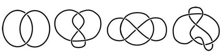
Fig 49 Left to right: Hopf link, figure-of-eight knot, Whitehead link, 6*2 knot.
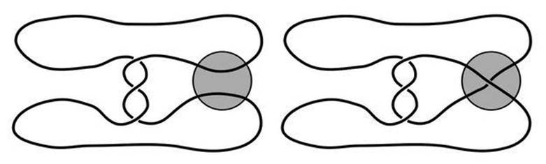
Fig 50 Action of enzyme Tn3 resolvase (grey circle) on a loop of DNA. Left: Before one application. Right: After.
Cozzarelli’s approach to this problem assumes that the enzyme makes the same change to the tangle topology each time it acts. This change can be viewed as tangle addition, with the same tangle being added each time. So we start with the unknot U and successively add a tangle X that represents the action of the enzyme, obtaining three tangle equations:
U + X = Hopf link
U + X + X = Figure-of-eight knot
U + X + X + X = Whitehead link
We then solve these for X. This, remarkably, is possible, and there is a unique answer. The tangle X has to act in exactly the way the schematic figure assumes. But this is no longer just the simplest guess, but a consequence of specific biological assumptions about the enzyme action, verified by experiment.
Can we make a prediction, a new experiment that will test whether the theory is correct? We can. Even more rarely, there ought to be a fourth action of the enzyme, leading to U+X+X+X+X. Since X is now known, we can work out which knot or link this is. It turns out to be a knot with no familiar name, which topologists call 6*2 (see Figure 49). The prediction, then, is that even less frequently than the triple reaction, we will observe the knot 6*2. And observations do indeed detect precisely this knot, with roughly the predicted degree of rarity.
Mathematical issues that sound fairly similar to those that arise with knots, but technically are very different, arise in a related area of molecular biology: protein folding. Although a protein is conceptually a chain of amino acids, in reality the chain folds up in a complex way under the influence of molecular forces. The basic point here is that the DNA, interpreted as amino acids, does not ‘contain the information’ that tells the protein how it should fold. Instead, the protein folds automatically, in response to the chemicals in the surrounding medium, the activity of special molecules called chaperonins which nudge it into particular configurations, temperature, and other factors.
Biologists often consider that anything passively obeying the laws of physics and chemistry is merely part of the background against which biology works. From that point of view, all that matters is that the physics does whatever the physics does. It can be taken for granted, even ignored. An elephant pushed off a cliff will fall – but that’s gravity, not biology. However, it is not possible to assign protein folding to this kind of background operation of physical law, because in principle proteins can fold in a huge variety of ways. Even if in practice they fold in only one way, we still need to know which shape arises, because a protein molecule’s shape is one of the main features that determine its biological function (or functions). Think of haemoglobin, which acts rather like molecular tongs, picking up a molecule of oxygen and putting it down again. If it weren’t the right shape, it couldn’t do the job. Figure 51shows how haemoglobin folds, and its two slightly different configurations.2
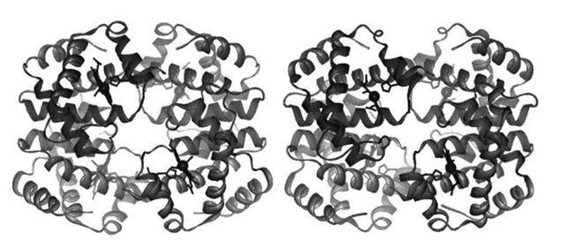
Fig 51 The two shapes of haemoglobin. Left: oxygen binds to regions shown as small dark spheres. Right: oxygen is released.
By the way, I’m not suggesting that haemoglobin is the only molecule that can transport oxygen.3 Tongs can have differently shaped handles without it impairing their function. Similarly, many other proteins could in principle transport oxygen. But any suitable molecule has to have a shape that lets it behave like oxygen-tongs. I mention this because it is sometimes suggested that haemoglobin is too complicated to have evolved – as if this specificmolecule were a target for evolution to aim at. On the contrary: evolution is opportunistic, and will settle for anything that works.
This role of shape is not just of theoretical importance. Many diseases, among them Creutzfeldt – Jakob disease, mad cow disease (BSE) and probably Alzheimer’s disease, may be caused by misfolded proteins. The ability to deduce the shape of a protein from its amino acid sequence would be a huge step forwards in biology, because sequencing DNA is now cheap and easy (if you have the rather expensive equipment and skills required) but working out the shape of a complicated protein is very hard.
The process was a huge puzzle until around 1990, when Joseph Bryngelson and Peter Wolynes at the University of Illinois devised a mathematical formulation in terms of an ‘energy landscape’. The forces that act between atoms and electrons in a molecule imply that any configuration of an amino acid chain (or any other molecule, for that matter) has a definite amount of energy. The mathematics and physics of dynamical systems imply that the molecule will behave in a manner that tries to make its energy as small as possible. Take an elastic band, and drop it on the desk. It tends to take up one particular unstretched shape. However, you can stretch the band into all sorts of shapes by pulling on different bits of it with your fingers. As you stretch it, though, you feel a certain amount of resistance. The more you stretch it, the harder you have to pull. What’s happening here is that in order to stretch the band, you have to increase its elastic energy. All the stretched shapes have more energy than the natural unstretched shape, and you have to do work to provide the extra energy. So the unstretched shape is the shape with the least energy.
It’s much the same with a protein molecule, but the different amino acids make it more like an elastic band with all sorts of lumps and bumps. Nevertheless, the stretched-out-straight shape has a lot of energy, and the protein molecule prefers to contract into a less energetic shape. In this way, nature can produce a specific shape of molecule by stitching amino acids together in turn, following the genetic instructions, and then just allowing the chain to fold itself into the required shape. Minimisation of energy does all the hard work, and the genes don’t need to tell the protein how to fold.
In the metaphor of an energy landscape, variations in energy of the conceivable configurations can be seen as hills and valleys, creating a conceptual landscape in which height corresponds to energy, and location in the landscape corresponds to the configuration concerned.
It is not practical to determine the actual shape of the protein by considering all possible shapes, working out the energy for each and seeing which is smallest, because the range of possible shapes is absolutely gigantic. It would be like trying to predict the shape of an elastic band by considering every conceivable shape, however implausible, computing the energy, and seeing which is smallest. This is not the only difficulty. I said that the molecule always ‘tries to make its energy as small as possible’, but that is an oversimplification. I should have said ‘as small as possible, compared with any nearby configuration’. The energy landscape may have a local depression, even though the lowest point on the entire landscape is far below that.
It is not only mathematicians who have trouble here. The molecule itself is much like the elastic band. It has no idea where the lowest point in the landscape is, so it heads downhill and finds out where that leads. If it leads into a local depression, the molecule gets trapped in the wrong configuration and the protein can’t do its job. In the late 1960s, Cyrus Levinthal, then a molecular biologist at Columbia University, realised that the energy landscape for a typical amino acid chain can have a gigantic number of possible local depressions.4 Suppose that the chain consists of 300 amino acids – which if anything is on the small side – and that the chemical bond linking each to the next can adopt one of a mere three stable angles. These angles are more or less independent, so the number of possible combinations is 3300, roughly 10143. This leads to Levinthal paradox: as a real protein chain folds, it cannot reach the ‘correct’ configuration by trying all possible configurations in turn. The universe will not last long enough.
The deduction is not that protein chains perform miracles, but that they don’t do it that way. A popular theory holds that evolution has eased the path: to ensure correct folding, the chains that are found in biologically significant proteins are not typical. Instead of having rough energy landscapes, with lots of bumps and hillocks, their landscapes form steep-sided funnels, with an obvious route down into the depths where the desired configuration lurks (see Figure 52). More precisely, they are made from a series of such funnels, each feeding the configuration into the next funnel along a specific path.5 The funnels are linked by saddle points – places which are local energy peaks in some directions and local depressions in others, like a mountain pass in a conventional landscape. The pass is the lowest point through which a traveller can cross a mountain ridge, so the path goes up to the pass and then descends, but the ridge itself rises upwards from the pass.
The idea is that natural selection will favour proteins with simple energy landscapes like this. Not because evolution somehow knows what the landscape looks like, but because molecules that often fold into a shape that doesn’t work will make the host organism less likely to survive, so these proteins will be weeded out.
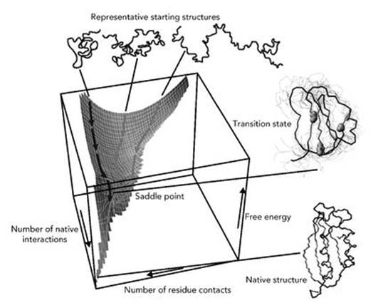
Fig 52 Energy landscape of a highly simplified model of a small protein, showing a deep funnel.
Even if this theory were right, the mathematics of protein folding would not become simple and straightforward, for other reasons. But at least we would understand how the molecule gets itself folded correctly.
Many different software packages make some kind of a stab at predicting how a protein will fold, using a mixture of mathematical principles and informed guesswork. A popular one is Rosetta, which harnesses the power of idle computers worldwide through its Rosetta@home project. This uses the Berkeley Open Infrastructure for Network Computing (BOINC) to carry out huge computations on a network provided by more than 80,000 volunteers, who allow the use of their home computers when they are not otherwise occupied. But in 2008 Seth Cooper and colleagues went one better, by turning protein folding into a multiplayer online computer game: Foldit. Players compete with one another and progress through increasing levels of difficulty, looking for the right way to fold a given protein.
Doing science using a computer game might seem an absurd piece of deference to popular culture, but it makes very effective use of something that humans have in abundance and computers lack: intuition. The human brain is very good at spotting patterns, even ones that it doesn’t consciously recognise. In 2010 Cooper’s team reported that ‘top-ranked Foldit players excel at solving challenging structural refinement problems’.6 The element of collaboration seems to add further power to the human brain’s intuitive understanding of three-dimensional shapes, and the competitive instinct provides motivation – as it does even in conventional science.
Foldit benefited from advice from professional game designers. Players progress by solving a series of puzzles, initially based on proteins whose structure is known, but not publicly available. Along the way they learn the many technical terms and techniques based on Rosetta, such as ‘combinatorial side-chain rotamer packing’, but using more friendly terminology – in this case, ‘shake’. Then they can progress to unsolved structures, with potential contributions to serious science.
Foldit is an intriguing example of a growing trend in science: getting the general public to participate in scientific research using distributed computing over the Internet. The problems have to be set up in an easily accessible way, but once this is done, a vast amount of computational power and human input becomes available – at very little cost. It’s a trend that could go a long way. As Zoran Popović, a project member, has said: ‘Our ultimate goal is to have ordinary people play the game and eventually be candidates for winning the Nobel prize.’
Foldit certainly beats Grand Theft Auto as a constructive way to pass the time, though it might not give you quite the same adrenaline rush.7