Mathematics of Life (2011)
Notes
Chapter 1: Mathematics and Biology
1 More precisely, the common house cat is Felis sylvestris catus, but its binomial name is Felis catus.
2 J.D. Watson and F.H. Crick, ‘Molecular structure of nucleic acids: a structure for deoxyribose nucleic acid’, Nature 171 (1953) 737 – 738.
3 The date depends on what you count as ‘completion’. A draft sequence was published in 2000, a so-called ‘complete’ draft in 2003. The sequence for the final chromosome, chromosome 1, was published in May 2006 in Nature.Some gaps remain, so it is arguable that the task is not yet finished. There are several thousand known gaps, inconsistencies and errors, currently being tidied up by a dedicated team of biologists.
Chapter 2: Creatures Small and Smaller
1 For an animation, see www.cellimagelibrary.org/images/8082
Chapter 3: Long List of Life
1 Most taxonomists consider Cyanistes to be a subgenus of the genus Parus, but the British Ornithologists’ Union considers it to be a distinct genus, on the basis of DNA sequencing (specifically, the mitochondrial DNA sequence of cytochrome B) which shows that these birds differ significantly from the other tits. As regards finer distinctions, C. caeruleus subdivides into at least nine subspecies.
Chapter 4: Florally Finding Fibonacci
1 H. Vogel, ‘A better way to construct the sunflower head’, Mathematical Biosciences 44 (1979) 179 – 189.
2 S. Douady and Y. Couder, ‘Phyllotaxis as a self-organised growth process’, in Growth Patterns in Physical Sciences and Biology (ed. J.-M. Garcia-Ruiz et al.), Plenum Press, New York (1993) 341 – 351.
3 L.S. Levitov, ‘Phyllotaxis of flux lattices in layered superconductors’, Physics Review Letters 66 (1991) 224 – 227; M. Kunz, ‘Some analytical results about two physical models of phyllotaxis’, Communications in Mathematical Physics 169 (1995) 261 – 295.
4 The species is Echinocactus grusonii inermis. See www.maths.surrey.ac.uk/hosted-sites/R.Knott/Fibonacci/fibnat.html#nonfib
5 G.W. Ryan, J.L. Rouse and L.A. Bursill, ‘Quantitative analysis of sunflower seed packing’, Journal of Theoretical Biology 147 (1991) 303 – 328.
6 P.D. Shipman and A.C. Newell, ‘Phyllotactic patterns on plants’, Physics Review Letters 92 (2004) 168102.
7 A.C. Newell, Zhiying Sun and P.D. Shipman, ‘Phyllotaxis and patterns on plants’, preprint, University of Arizona 2009.
Chapter 5: The Origin of Species
1 ‘Presidential Address’, Proceedings of the Linnaean Society, 24 May (1859) viii.
2 F. Darwin (ed.), The Foundations of The Origin of Species. Two essays written in 1842 and 1844. Cambridge University Press, Cambridge (1909).
3 At first sight it is difficult for a modern mind to understand how anyone could arrive at such a specific date. The Book of Genesis, for instance, does not tell us how long Adam and Eve lived in the Garden of Eden before being expelled. But Ussher’s deductions from genealogical records in the Old Testament convinced him that the date of creation was precisely 4,000 years before the birth of Christ. If Ussher could date the nativity accurately, he would automatically date the creation. At that time the consensus among theologians was that Jesus was born in 4 BC, hence 4004 BC for the Creation. Ussher could date other Biblical events as well: Noah’s flood, he found, occurred in 2348 BC.
4 A survey by Gallup in 2004 indicated that about 45% of Americans accept both a 10,000-year-old Earth and the divine origin of the planet, 38% assigned the Earth’s origin to God but preferred a timescale of millions of years, and 13% believed that it took millions of years and God played no part in the process. In a 1997 Gallup poll of Americans with science degrees, only 5% thought that the Earth was less than 10,000 years old. Another 40% accepted divine creation, but placed it millions of years in the past. The remaining 55% believed that the Earth was extremely ancient, and that God played no role in the evolution of humans. Among those earning less than $20,000 per year, the corresponding figures were 59%, 28% and 6.5%; among those earning more than $50,000 per year they were 29%, 50% and 17%.
5 The poem was written in 1849, twenty years before the Origin appeared. But it was influenced by the 1844 book Vestiges of the Natural History of Creation, published anonymously by Robert Chambers. This book described the transmutation of species, the evolution of stars and other speculative scientific theories, and softened up public opinion for later ideas about evolution. It found favour with radicals, but once its implications had sunk in, it was denounced by the establishment for its alleged materialism.
6 Think of football. Ignoring draws, one team must win and one team must lose in each match. But winning is not purely random. Teams that have greater skill with the ball tend to win more matches. If we define ‘skill’ tautologously, in terms of which team wins, the above statement will still be true. However, that’s the start of understanding, not the end. On closer examination we can discover which abilities with the ball, or strategy, or strength, or passion or ‘belief’ make teams more likely to win than others. If we could kill off losing teams, and clone winning ones, along with their skills, the standard of play would generally improve.
Louis Amaral used network methods to analyse the skills of teams in the 2008 UEFA European Football Championship, assigning points for precision in passing, shots at goal, and so on. These data, derived from video footage of the games, were used to assign a skill level to each team. This ranking closely matched the actual results in the tournament. See J. Duch, J.S. Waitzman and L.A.N. Amaral, ‘Quantifying the performance of individual players in a team activity’, PLoS ONE 2010 5(6): e10937. doi:10.1371/journal.pone.0010937.
7 Two small herbivorous dinosaurs are happily eating plants when they spot an approaching velociraptor. (It used to be tyrannosaur, but we are in the post-Jurassic Park era now.) One of them immediately starts to run. ‘There’s no point in running away,’ says the other. ‘You can’t outrun a velociraptor.’ The first one turns and shouts back over its shoulder, ‘No, but I can run faster than you!’
8 Actually, this is a simplification. Some regions of the genome are more likely to change than others, for instance.
9 Theodosius Dobzhansky, ‘Nothing in biology makes sense except in the light of evolution’, American Biology Teacher 35 (1973) 125 – 129.
10 In 1841 Richard Owen, a leading palaeontologist, found an incomplete fossil that he thought was a hyrax (because of its teeth) and assigned it to a new genus, Hyracotherium. In 1876 Othniel Marsh, Owen’s rival, discovered a complete skeleton, obviously horse-like, and assigned it to another new genus, Eohippus (dawn horse). Later it became clear that the two fossils belonged to the same genus, and by the rules of taxonomy the name that was the first to be published won. So the evocative ‘dawn horse’ was lost, and a scientific misconception was preserved.
Chapter 6: In a Monastery Garden
1 Perhaps too well: reanalysis of Mendel’s data suggests that the fit is better than we should expect statistically. Perhaps there was some subconscious massaging of the data in ambiguous cases. See R.A. Fisher, ‘Has Mendel’s work been rediscovered?’, Annals of Science 1 (1936) 115 – 137.
2 This convention is not obvious. Usually the symbols are standardised so that in AB the factor A comes from the father and B from the mother, so AB and BA are potentially distinguishable. Mendel’s experiments were what suggested that AB=BA.
Chapter 7: The Molecule of Life
1 Originally deoxyribose nucleic acid. See the quote from Crick and Watson on p. 6.
2 This may seem a chicken-and-egg situation: you need DNA to specify the enzymes, and you need the enzymes to copy DNA. Like all such puzzles, the answer is presumably that this feedback loop had simpler origins, without this recursive structure.
3 Mitochondria of animals or microorganisms (but not plants) use UGA (U=uracil) to encode tryptophan rather than STOP. When translated by the cell’s molecular machinery, synthesis stops where tryptophan should have been inserted. In addition, most animal mitochondria use AUA for methionine, not isoleucine; vertebrate mitochondria use AGA and AGG as STOP, and yeast mitochondria assign all triplets beginning with CU to threonine instead of leucine.
4 Richard Dawkins, The Selfish Gene, Oxford University Press, Oxford (1989).
5 Meaning ‘we don’t understand what this bit does’, and typically confused with ‘this bit does nothing’.
6 A bizarre misconception sometimes inspired by this term is that your DNA makes you selfish.
7 Jack Cohen and Ian Stewart, The Collapse of Chaos, Viking, New York (1994).
8 John S. Mattick, ‘The hidden genetic program of complex organisms’, Scientific American, October 2004, 291(4) 60 – 67.
Chapter 8: The Book of Life
1 US Governmental agencies have a long track record of funding research that seems outside their natural remit. The project was handled by a special subcommittee of the DoE’s Health and Environmental Research Advisory Committee.
2 In 2010 a US court ruled that nine patents filed by a company called Myriad, related to the so-called breast cancer genes BRCA1 and BRCA2, are invalid. As I write, the decision is being appealed.
3 At least not yet. But nanotechnology opens up the possibility of pulling a strand of DNA through a device that can read off the bases by exploiting subtle differences in their electronic properties. Some progress has already been made; the latest is to make a small hole in a layer of graphene, which is a honeycomb of carbon atoms just one atom thick.
4 T. Radford, “‘Gay gene” theory fails blood test’, The Guardian (23 April 1999) 11.
5 D.H. Hamer, S. Hu, V.L. Magnusson, N. Hu and A.M. Pattatucci, ‘A linkage between DNA markers on the X chromosome and male sexual orientation’, Science 261 (1993) 321 – 327.
6 G. Rice, C. Anderson, N. Risch and G. Ebers, ‘Male homosexuality: absence of linkage to microsatellite markers at Xq28’, Science 284 (1999) 665 – 667.
Chapter 9: Taxonomist, Taxonomist, Spare that Tree
1 K. Ochiai, T. Yamanaka, K. Kimura and O. Sawada. ‘Inheritance of drug resistance (and its transfer) between Shigella strains and between Shigella and E. coli strains’ [in Japanese], Hihon Iji Shimpor 1861 (1959) 34.
2 D.L. Theobald, ‘A formal test of the theory of universal common ancestry’, Nature 466 (2010) 219 – 222.
Chapter 10: Virus from the Fourth Dimension
1 Euclid put geometry on a systematic basis, but he seems not to have created much new geometry of his own. Other Greek geometers, such as Apollonius, Eudoxus and Archimedes, are generally considered to have been more creative as mathematicians.
2 The cube can also be called a hexahedron, keeping the names consistent, but nobody does that any more.
3 For example, Archimedes’ principle remains fundamental in the design of ships, because it governs whether they will float, and if so, how stable they will be. And the law of the lever is built into computer software for designing buildings, cars and bridges.
4 Ian Stewart, Why Beauty is Truth, Basic Books, New York (2007).
5 D.L.D. Caspar and A. Klug, ‘Physical principles in the construction of regular viruses’, Cold Spring Harbor Symposia on Quantitative Biology 27, Cold Spring Harbor Laboratory, New York (1962) 1 – 24.
6 N.G. Wrigley, ‘An electron microscope study of the structure of Sericesthis iridescent virus’, Journal of General Virology 5 (1969) 123 – 134; N.G. Wrigley, ‘An electron microscope study of the structure of Tipula iridescent virus’, Journal of General Virology 5 (1970) 169 – 173.
7 R.C. Liddington, Y. Yan, J. Moulai, R. Sahli, T.L. Benjamin and S.C. Harrison, ‘Structure of simian virus 40 at 3.8-Å resolution’, Nature 354 (1991) 278 – 284.
8 R. Twarock, ‘A mathematical physicist’s approach to the structure and assembly of viruses’, Philosophical Transactions of the Royal Society of London A 364 (2006) 3357 – 3374.
9 R. Twarock, ‘A tiling approach to virus capsid assembly explaining a structural puzzle in virology’, Journal of Theoretical Biology 226(4) (2004) 477 – 482.
10 If you’re wondering how Donald is extracted from H.S.M., the M stands for MacDonald.
Chapter 11: Hidden Wiring
1 S. Herculano-Houzel, B. Mota and R. Lent, ‘Cellular scaling rules for rodent brains’, Proceedings of the National Academy of Sciences 103 (2006) 12138 – 12143; S. Herculano-Houzel, ‘The human brain in numbers: a linearly scaled-up primate brain’, Frontiers in Human Neuroscience 3 (2009) article 31.
2 A. Hodgkin and A. Huxley, ‘A quantitative description of membrane current and its application to conduction and excitation in nerve’, Journal of Physiology 117 (1952) 500 – 544.
3 The Hodgkin – Huxley equations take the form
![]()
where I=membrane current, C=membrane capacitance, V=voltage, VK, VNa and VL are constants related to the potassium, sodium and other ion channels, and m, n and h are determined by three differential equations based on observed data.
4 The FitzHugh – Nagumo equations (with no applied current) are:
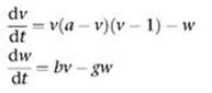
where v is a dimensionless form of the voltage V, and w combines the roles of m, n and h in the Hodgkin – Huxley equations into a single variable.
5 M. Golubitsky, I. Stewart, P.-L.Buono and J.J. Collins, ‘Symmetry in locomotor central pattern generators and animal gaits’, Nature 401 (1999) 693 – 695.
6 C.A. Pinto and M. Golubitsky, ‘Central pattern generators for bipedal locomotion’, Journal of Mathematical Biology 53 (2006) 474 – 489.
7 R.L. Calabrese and E. Peterson, ‘Neural control of heartbeat in the leech Hirudo medicinalis’ in Neural Origin of Rhythmic Movements (ed. A. Roberts and B. Roberts), Symposium of the Society for Experimental Biology 37(1983) 195 – 221; E. De Schutter, T.W. Simon, J.D. Angstadt and R.L. Calabrese, ‘Modeling a neuronal oscillator that paces heartbeat in the medicinal leech’, American Zoologist 33 (1993) 16 – 28; R.L. Calabrese, F. Nadim and Ø.H. Olsen, ‘Heartbeat control in the medicinal leech: a model system for understanding the origin, coordination, and modulation of rhythmic motor patterns’, Journal of Neurobiology 27 (1995) 390 – 402; W.B. Kristan Jr, R.L. Calabrese and W.O. Friesen, ‘Neuronal control of leech behavior’, Progress in Neurobiology 76 (2005) 279 – 327.
8 P.-L. Buono and A. Palacios, ‘A mathematical model of motorneuron dynamics in the heartbeat of the leech’, Physica D 188 (2004) 292 – 313.
9 H.R. Wilson and J.D. Cowan, ‘Excitatory and inhibitory interactions in localized populations of model neurons’, Biophysical Journal 12 (1972) 1 – 24.
10 P.C. Bressloff, J.D. Cowan, M. Golubitsky and P.J. Thomas, ‘Scalar and pseudoscalar bifurcations motivated by pattern formation on the visual cortex’, Nonlinearity 14 (2001) 739 – 775; P.C. Bressloff, J.D. Cowan, M. Golubitsky, P.J. Thomas and M.C. Wiener, ‘Geometric visual hallucinations, Euclidean symmetry, and the functional architecture of striate cortex’, Philosophical Transactions of the Royal Society of London B 356 (2001) 299 – 330; P.C. Bressloff, J.D. Cowan, M. Golubitsky, P.J. Thomas and M.C. Wiener, ‘What geometric visual hallucinations tell us about the visual cortex’, Neural Computation 14 (2002) 473 – 491.
11 J.W. Zweck and L.R. Williams, ‘Euclidean group invariant computation of stochastic completion fields using shiftable – twistable functions’, Journal of Mathematical Imaging and Vision 21 (2004) 135 – 154.
Chapter 12: Knots and Folds
1 S.A. Wasserman, J.M. Dungan and N.R. Cozzarelli, ‘Discovery of a predicted DNA knot substantiates a model for site-specific recombination’, Science 229 (1985) 171 – 174; D. Sumners, ‘Lifting the curtain: using topology to probe the hidden action of enzymes’, Notices of the American Mathematical Society 42 (1995) 528 – 537.
2 Animations showing how haemoglobin changes shape when binding to oxygen, or releasing it, can be found at en.wikipedia.org/wiki/ Hemoglobin#Binding_for_ligands_other_than_oxygen.
3 I’m simplifying a complicated tale by talking of haemoglobin as if it were unique. Actually, many variants of the specific form of haemoglobin shown in Figure 51 exist in nature. They are all fairly similar and probably have a common evolutionary origin. The point is stronger: in principle, vast numbers of radically different molecules could also transport oxygen. ‘The right shape’ here doesn’t mean ‘the only shape’: it means any shape that will do the job. Lots will; far more won’t.
4 C. Levinthal, ‘How to fold graciously’, in Mössbauer Spectroscopy in Biological Systems (ed. J.T.P. DeBrunner and E. Munck), University of Illinois Press, Illinois (1969) 22 – 24.
5 C.M. Dobson, ‘Protein folding and misfolding’, Nature 426 (2003) 884 – 890.
6 S. Cooper, F. Khatib, A. Treuille, J. Barbero, J. Lee, M. Beenen, A. Leaver-Fay, D. Baker, Z. Popović and Foldit players, ‘Predicting protein structures with a multiplayer online game’, Nature 466 (2010) 756 – 760.
7 You can try Foldit for yourself at http://fold.it/portal/
Chapter 13: Spots and Stripes
1 A.M. Turing, ‘The chemical basis of morphogenesis’, Philosophical Transactions of the Royal Society of London B 237 (1952) 37 – 72.
2 J. Murray, Mathematical Biology, Springer, Berlin (1989).
3 S. Kondo and R. Asai, ‘A reaction – diffusion wave on the skin of the marine angelfish Pomacanthus’, Nature 376 (1995) 765 – 768.
4 The precise statement of ‘a lot of symmetry’ is called the maximal isotropy subgroup conjecture. This plausible conjecture was eventually proved false: see M.J. Field and R.W. Richardson, ‘Symmetry breaking and the maximal isotropy subgroup conjecture for reflection groups’, Archive for Rational Mechanics and Analysis 105 (1989) 61 – 94.
5 H. Meinhardt, ‘Models of segmentation’, in Somites in Developing Embryos (ed. R. Bellairs et al.), Nato ASI Series A 118, Plenum Press, New York (1986) 179 – 189.
6 P. Eggenberger Hotz, ‘Combining development processes and their physics in an artificial evolutionary system to evolve shapes’, in On Growth, Form, and Computers (ed. S. Kumar and P.J. Bentley), Elsevier, San Diego CA (2003) 302 – 318.
Chapter 14: Lizard Games
1 J. Maynard Smith, Evolution and the Theory of Games, Cambridge University Press, Cambridge (1982) 16.
2 M. Pigliucci, ‘Species as family resemblance concepts: the (dis-)solution of the species problem?’, BioEssays 25 (2003) 596 – 602.
3 N. Knowlton, ‘Sibling species in the sea’, Annual Review of Ecology and Systematics 24 (1993) 189 – 216.
4 This is not straightforward, and some aspects are controversial. Some regions of the genome are conserved by natural selection: even if mutations happen, they don’t survive.
5 L.M. Mathews and A. Anker, ‘Molecular phylogeny reveals extensive ancient and ongoing radiations in a snapping shrimp species complex (Crustacea, Alpheidae, Alpheus armillatus)’, Molecular Phylogenetics and Evolution 50(2009) 268 – 281.
6 G. Vogel, ‘African elephant species splits in two’, Science 293 (2001) 1414.
7 H. Sayama, L. Kaufman and Y. Bar-Yam, ‘Spontaneous pattern formation and genetic diversity in habitats with irregular geographical features’, Conservation Biology 17 (2003) 893; M.A.M. de Aguiar, M. Baranger, Y. Bar-Yam and H. Sayama, ‘Robustness of spontaneous pattern formation in spatially distributed genetic populations’, Brazilian Journal of Physics 33 (2003) 514 – 520.
8 A.S. Kondrashov and F.A. Kondrashov, ‘Interactions among quantitative traits in the course of sympatric speciation’, Nature 400 (1999) 351 – 354.
9 U. Dieckmann and M. Doebeli, ‘On the origin of species by sympatric speciation’, Nature 400 (1999) 354 – 357.
10 The species of Darwin’s finch are:
Large cactus-finch, Geospiza conirostris
Sharp-beaked ground-finch, Geospiza difficilis
Vampire finch, Geospiza difficilis septentrionalis [subspecies]
Medium ground-finch, Geospiza fortis
Small ground-finch, Geospiza fuliginosa
Large ground-finch, Geospiza magnirostris
Darwin’s large ground-finch, Geospiza magnirostris magnirostris [possibly
extinct subspecies]
Common cactus-finch, Geospiza scandens
Vegetarian finch, Camarhynchus crassirostris
Large tree-finch, Camarhynchus psittacula
Medium tree-finch, Camarhynchus pauper
Small tree-finch, Camarhynchus parvulus
Woodpecker finch, Camarhynchus pallidus
Mangrove finch, Camarhynchus heliobates
Warbler finch, Certhidea olivacea
11 That term was made popular by the second book, but it originated with Percy Lowe in 1936.
12 More precisely, the mean phenotype changes continuously, even though the two new phenotypes appear through jumps. If we consider how phenotypes deviate from their average values, the word ‘unchanged’ applies, and this is what the mathematical models actually study. J. Cohen and I. Stewart, ‘Polymorphism viewed as phenotypic symmetry breaking’, in Nonlinear Phenomena in Biological and Physical Sciences (ed. S.K. Malik et al.), Indian National Science Academy, New Delhi (2000) 1 – 63; I. Stewart, T. Elmhirst and J. Cohen, ‘Symmetry breaking as an origin of species’, in Bifurcations, Symmetry, and Patterns (ed. J. Buescu et al.), Birkhäuser, Basel (2003) 3 – 54.
Chapter 15: Networking Opportunities
1 A. Tero, S. Takagi, T. Saigusa, K. Ito, D.P. Bebber, M.D. Fricker, K. Yumiki, R. Kobayashi and T. Nakagaki, ‘Rules for biologically inspired adaptive network design’, Science 327 (2010) 439 – 442.
2 Translating his symbolic terminology into features of the diagram, what matters is how many lines meet at a given dot. Suppose, for example, that a closed path exists. Then whenever the path runs into a dot, it also departs from that dot. So the number of lines meeting any given dot must be even. This disposes of the Königsberg bridges, because the diagram has three dots where three lines meet, and one dot where five lines meet. Since the number of lines is odd in these cases, the puzzle cannot be solved with a closed path. Open paths have two distinct ends, and at each of these the number of lines running into the dot is odd. Everywhere else, it is even. So now there must be exactly two dots that meet an odd number of lines: one at each end of the path. Since the Königsberg diagram has four dots meeting an odd number of lines, there is no open path either.
Euler proved that these conditions are also sufficient for a path of the appropriate kind to exist provided the diagram is connected (any two dots are joined by some path). Euler devotes several pages to a symbolic proof; in diagrammatic form it can be made virtually obvious.
3 Y. Kuramoto, Chemical Oscillations, Waves, and Turbulence, Springer, New York (1984).
4 J.R. Collier, N.A.M. Monk, P.K. Maini and J.H. Lewis, ‘Pattern formation by lateral inhibition with feedback: a mathematical model of Delta – Notch intercellular signalling’, Journal of Theoretical Biology 183 (1996) 429 – 446.
Chapter 16: The Paradox of the Plankton
1 Specifically, it is the integer closest to ![]() where φ is the
where φ is the
2 The equation is
![]()
where r and N are constants; here we can interpret r as the unconstrained growth rate, and K is the maximum population size. The actual growth rate, at population N, is r(1-N/K), which depends on N: such a growth rate is said to be density-dependent.
With initial conditions N(0)=N0, the logistic equation can be solved explicitly by standard methods, and the solution is
![]()
where N0 is the initial population.
3 R.M. May, ‘Simple mathematical models with very complicated dynamics’, Nature 261 (1976) 459 – 467.
4 The trick is to scale Xt to bXt/a.
5 The model is:
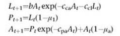
where Lt is the number of feeding larvae, Pt is the number of non-feeding larvae, pupae and newly emerged adults, and At is the number of adults, all at time t. The other symbols are parameters.
6 Period-2: R.F. Costantino, J.M. Cushing, B. Dennis and R.A. Desharnais, ‘Experimentally induced transitions in the dynamic behavior of insect populations’, Nature 375 (1995) 227 – 230; Chaos: R.F. Costantino, R.A. Desharnais, J.M. Cushing and B. Dennis, ‘Chaotic dynamics in an insect population’, Science 275 (1997) 389 – 391.
7 J. Huisman and F.J. Weissing, ‘Biodiversity of plankton by species oscillations and chaos’, Nature 402 (1999) 407 – 410.
8 E. Benincà, J. Huisman, R. Heerkloss, K.D. Jöhnk, P. Branco, E.H. Van Nes, M. Scheffer and S.P. Ellner, ‘Chaos in a long-term experiment with a plankton community’, Nature 451 (2008) 822 – 825.
9 M.J. Keeling, ‘Models of foot-and-mouth disease’, Proceedings of the Royal Society of London B 272 (2005) 1195 – 1202.
Chapter 17: What is Life?
1 There was a forerunner, called Project Ozma, in 1960.
2 For a full specification see en.wikipedia.org/wiki/ Von_Neumann_cellular_automata
3 J. Von Neumann and A.W. Burks, Theory of Self-Reproducing Automata, University of Illinois Press, Chicago (1966).
4 See e.g. www.ibiblio.org/lifepatterns/
5 E.R. Berlekamp, J.H. Conway and R.K. Guy, Winning Ways volume 2, Academic Press, London (1982).
6 M. Cook, ‘Universality in elementary cellular automata’, Complex Systems 15 (2004) 1 – 40.
7 C.G. Langton, ‘Artificial life’, in Artificial Life (ed. C.G. Langton), Addison-Wesley, Reading MA (1989), 1.
8 www.darwinbots.com/WikiManual/index.php/Main_Page
9 ‘Smallest’ here is usually interpreted as ‘take any more DNA away and it won’t work’. Such a genome need not be unique, because there might be several different ways to cut a genome down to size, each working for different reasons.
Chapter 18: Is Anybody Out There?
1 K. Thomas-Keprta, S. Clemett, D. McKay, E. Gibson and S. Wentworth, ‘Origin of magnetite nanocrystals in Martian meteorite ALH 84001’, Geochimica et Cosmochimica Acta 73 (2009) 6631 – 6677.
2 D. Brownlee and P.D. Ward, Rare Earth, Copernicus, New York (2000).
3 Both words are Latin – Greek hybrids, which used to be unacceptable but are now so common that few object to them. ‘Television’ is a case in point.
4 Let there be n planets, with n large, and let p = 1/n. The binomial distribution tells us that the probability of getting exactly one planet with intelligent life is np(1-p)n-1, which is very close to e-1 because np=1 and (1-1/n)n-1 is close to e-1. Here e=2.718 is the base of natural logarithms, so e-1=0.37. The probability of no such planets is (1-p)n, which is the same. The probability of two or more is 1-0.37-0.37=0.26.
5 ‘Currently’ may seem to contradict relativity, which says that no concept of simultaneity can be consistent for all inertial observers. That may be true, but we can adopt a privileged frame of reference – our own. The intelligent aliens can then be current from our point of view.
6 C.D.B. Bryan, Close Encounters of the Fourth Kind, Alfred A. Knopf, New York (1995).
7 G. Wächtershäuser, ‘Groundworks for an evolutionary biochemistry: the iron – sulphur world’, Progress in Biophysics and Molecular Biology 58 (1992) 85 – 201.
8 N. Lane, ‘Genesis revisited’, New Scientist 2772 (17 August 2010) 36 – 39.
9 O.U. Mason, T.Nakagawa, M. Rosner, J.D. Van Nostrand, J. Zhou, A. Maruyama, M.R. Fisk and S.J. Giovannoni, ‘First investigation of the microbiology of the deepest layer of ocean crust’, PlosOne, 5(11): e15399.doi:10.1371/journal.pone.0015399.
10 This was the number on 11 January 2011.
11 M.R. Swain, G. Vasisht and Giovanna Tinetti, ‘The presence of methane in the atmosphere of an extrasolar planet’, Nature 452 (2008) 329 – 331.
12 J.L. Bean, E.M.-R. Kempton and D. Homeier, ‘A ground-based transmission spectrum of the super-Earth exoplanet GJ 1214b’, Nature 468 (2010) 669 – 672.
13 J. Laskar, F. Joutel and P. Robutel, ‘Stabilization of the Earth’s obliquity by the Moon’, Nature 361 (1993) 615 – 617.
14 The Apollo Moon missions brought back rocks which show that the Moon’s surface has much the same composition as the Earth’s mantle. The Moon also has a large angular momentum. An attractive way to explain both these facts is a collision between the Earth and another large body, which splashed off a big chunk of mantle, forming the Moon. Simulations show that a Mars-sized body could have done this. This ‘giant impact hypothesis’ became established, and the body concerned was named Theia. But later, improved simulations show that a big chunk of Theia ends up on the Moon too. So now it is assumed that Theia had almost exactly the same composition as the Earth’s mantle. This puts us back where we were at the start, but with an extra body involved. I call this ‘losing the plot’.
15 I’m simplifying the discussion slightly: the usual formula also includes the planet’s emissivity – its ability to emit radiation. I’ve set that to the value 1, which is typical. The formula is
![]()
where Tp is the temperature of the planet, Ts is the temperature of the star, R is the radius of the star, D is the distance from the star to the planet, α is the planet’s albedo and ε is the planet’s emissivity.
For the Sun – Earth system, Ts=5,800 K, R=700,000 km, α=0.3, and the Earth’s average emissivity in the infrared region of the spectrum (which is where most of the energy is radiated away) is approximately given by ε=1. Substituting these figures into the formula yields Tp=254 K.
16 An example is the exoplanet HD 209458b.
17 The metalloid magma-dwellers of Grumbatula VI used to think that Sol III (the Earth) was far too cold to support life, being well outside the habitable zone of the Sun in which the surfaces of planets are molten rock. The discovery of Earth’s subterranean magma ocean, containing a million times as much magma as all the oceans of Grumbatula VI put together, was at first greeted with incredulity because there was no conceivable heat source to keep it molten, but has now provoked a rethink among the more imaginative astroscholars.
18 M. Dellnitz, K. Padberg, M. Post and B. Thiere, ‘Set oriented approximation of invariant manifolds: review of concepts for astrodynamical problems’, in New Trends in Astrodynamics and Applications III (ed. E. Belbruno), AIP Conference Proceedings 886 (2007) 90 – 99.
19 D. Sasselov and D. Valencia, ‘Planets we could call home’, Scientific American 303(2) (August 2010) 38 – 45.