Methods of Mathematics Applied to Calculus, Probability, and Statistics (1985)

Part II. THE CALCULUS OF ALGEBRAIC FUNCTIONS

Chapter 11. Integration

11.1 HISTORY

The integral calculus was actually developed before the differential calculus. It arose from the problem of finding areas and volumes defined by mathematical expressions. In the early stages each particular area or volume problem was solved by a suitable trick. The great progress occurred when systematic methods were introduced and the fundamental theorem of the calculus was discovered. This theorem says that differentiation and integration are inverse processes one to the other (much as multiplication and division are inverse processes).

Experience seems to show that when presenting the calculus for the first time it is preferable to put the differential calculus before the integral calculus (which is what we have done). Nevertheless, mathematically it is the other way around; the rigorous approach is easiest from the integration side. We will base our approach to the integral calculus on the idea of area, and then extend, generalize if you prefer, the idea to a broader context. It is necessary, therefore, to first review your beliefs about area.

11.2 AREA

You emerge from elementary Euclidean geometry with the belief that the area of a square is proportional to the square of the side. For example, you can see directly that a square 10 by 10 is composed of 100 congruent unit squares (Figure 11.2-1). It is conventional to take the constant of proportionality as being 1. Hence, the measure of the area of a square is the square of the side.

Next, you believe that the area of a finite sum of nonoverlapping areas is the sum of the individual areas, in short that area is additive for finite sums of areas. Along the way you also agree that area is to be measured by a positive number, with 0 being the area of “nothing.”

You also believe that congruent figures must have the same area; you would be logically embarrassed if you did not, since congruent figures are interchangeable as far as area is concerned.

Finally, and this is an assumption, too, you probably believe that every figure has a unique area. This means, for example, that you are assured, when you compute it, that the area of a triangle is independent of which side you pick for the base.

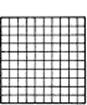
Figure 11.2-1 A 10 by 10 square

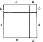
Figure 11.2-2 Square (a + b)²

Looking at Figure 11.2-2, you can see that the algebraic identity

A = (a + b)² = a² + 2ab + b²

corresponds to a geometric identity. This identity says that the whole square is the sum of the two squares (of area a² and b²), plus the two, congruent rectangles. The two congruent rectangles have necessarily the same area. From this you deduce that the area of a single rectangle of sides a and b must be

A = ab

The diagonal of a rectangle (Figure 11.2-3) divides it into two congruent triangles, and therefore each of these right triangles must have the area

Now any triangle, right or otherwise, can have a perpendicular dropped from a vertex to the base, which cuts the given triangle into two right triangles (Figure 11.2-4). You can either make sure that the vertex chosen is the largest angle, or else discuss the fact that, if the perpendicular (the altitude) falls outside the triangle then you are talking about the difference between the areas of the two triangles. Either way, from the assumptions you come fairly directly to the formula for the area of a general triangle:

Figure 11.2-3 Rectangle as two triangles

Figure 11.2-4 Triangle

Next, any plane closed figure that does not cross itself and is bounded by a finite number of straight lines may be decomposed into triangles (Figure 11.2-5). At any convex angle (less than 180° as seen from the inside of the region, and there is always at least one such angle), you can, as in Figure 11.2-6, reduce the number of sides by 1 when you draw the third side of the triangle since what is left to triangulate has one less side. The triangulation is not unique (but you can see that it can always be done). Since you assumed that the area is unique, it does not matter just how the triangle decomposition is done; the resulting area will be the same for a given figure (again, having a finite number of sides).

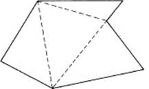
Figure 11.2-5

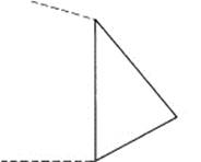
Figure 11.2-6

It is when you face the area of a circle, for example, that you need to think. It soon becomes evident that some new definition, an extension of the old definition, of area must be made for regions bounded by other than straight lines. No matter how you choose to extend the definition, it should be consistent with the earlier definition. In short, it is necessary to make an extension of area to new shapes, a standard situation in creating new mathematics.

EXERCISE 11.2

1.Draw a right triangle and drop a perpendicular from the right angle to the hypotenuse. This divides the original triangle T₁ into two triangles T₂ and T₃. The three triangles are similar. Derive Pythagoras’ theorem.

11.3 THE AREA OF A CIRCLE

The simplest figure that has curved sides is the circle. While Euclid’s Elements proves that the areas of circles are to each other as the squares of their respective sides, nowhere does he discuss the number π; nowhere does he get the measure of the area.

The historical approach to finding the area of a circle is to inscribe (inscribe means draw inside) a regular polygon in the circle and then compute the area of the polygon. This area is taken to be a lower bound on the area of the circle. Archimedes by a clever device doubled the number of sides of the inscribed polygon (see Figure 11.3-1). Then he again doubled the number of sides, and so on. He then took the limit of the area of the sequence of inscribed polygons to be the area of the circle.

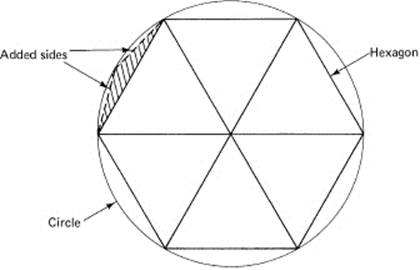
Figure 11.3-1

There were endless arguments as to whether the polygon became the circle in the limit or not. There was confusion between (1) the area of the inscribed polygons approaching the area of the circle, and (2) various properties of the perimeter (straight line segments) approaching a constantly curving circle. We have learned to avoid such questions and confine ourselves to the question, “Does the area of the inscribed polygons get arbitrarily close to the area of the circle?”

But we are not as sure as we might be when we merely use this approach of inscribing regular polygons; instead, we propose to also circumscribe (circum-, around) a regular polygon around the outside of the circle (Figure 11.3-2) and again let the number of sides be doubled indefinitely. If the two areas, that of the inscribed and that of the circumscribed polygons, approach the same number, then it seems reasonable to take this common number as the area of the circle. Note that we are actually defining what we mean by the area of a figure with curved sides.

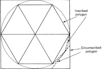
Figure 11.3-2

This approach is a tedious piece of special algebra and trigonometry to carry out for a circle. What is important is both the plan for finding a common limit and the realization that a new definition is required to deal with areas bounded by curved lines. Instead of finding the area of a circle, we will start finding the areas under the parabolas (a generalization of y = x²),

y = cx^k (k >0)

and later (Examples 11.9-4 and 16.7-1) find the area of a circle in a simple fashion.

11.4 AREAS OF PARABOLAS

Example 11.4-1

Given the family of parabolas

the simplest case, k = 1, is a straight line. This forms a triangle whose area we already know (we can use this case as a check on what we are doing). We have

y = cx

To estimate the area under the curve, above the x-axis, and to the left of the vertical line x = a, we first inscribe (see Figure 11.4-1) a sequence of narrow rectangles, and then examine the limit as the number of rectangles approaches infinity (gets arbitrarily large). Take the width of each rectangle to be

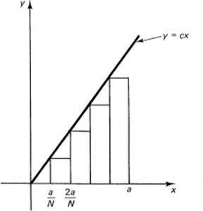
Figure 11.4-1

where N = the number of rectangles. From the figure we have the inscribed area A_I(N) [A_I(N) depends on N, of course].

But this can be simplified by factoring ac/N from each term:

We know the sum of the consecutive integers from Section 2.3 (N – 1 = n in the formula), and we also can eliminate the Δx = a/N. We get the area of the inscribed polygons:

Rearranging this, we have

and this approaches the limit A₁:

as N approaches infinity. We recognize that this is the correct answer for a triangle. But let. us persevere in our approach and compute the area of the circumscribed set of rectangles.

For the circumscribed set of rectangles, we get exactly the same thing (see Figure 11.4-2), except that the sequence of rectangles begins with the height proportional to 1 and goes on to height proportional to N, instead of beginning with the 0 and going to N – 1. We have, therefore [compare with Equation (11.4-2)], the circumscribed area

and the corresponding sum is [compare with Equation (11.4-3)]

Rearranging this, we have

which again approaches (11.4-4):

Thus the limit of both the inscribed and the circumscribed areas is the same. We have tested the approach on a known result and found that it works correctly.

When you consider the difference between the inscribed and circumscribed sums, (11.4-5) and (11.4-6), you see that it is

and that as N → ∞ the difference must approach zero.

Example 11.4-2

The next case is k = 2,

y = x²

We have chosen to ignore the front constant c (since from Example 11.4-1 you see that it will simply factor out of everything, and remain in front of the final answer). From Figure 11.4-3 you have the inscribed area under the curve, above the x-axis, and to the left of the line x = a. The area is

After factoring out the common factors and replacing Δx by its proper value (a/N) in terms of N, you have [compare with (11.4-2)]

The circumscribed area is correspondingly [compare with (11.4-5)]

(the difference being again the end terms). For the inscribed area, from Example 2.3-2, we have, on substituting for the sum of the squares of the consecutive integers (n = N – 1),

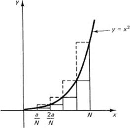
Figure 11.4-2

and for the circumscribed area (n = N),

It is easy to see that as N → ∞ both expressions approach

Thus we take a³/3 as the area under the second-degree parabola. From these two examples (plus just plain thinking), we are inclined to accept the definition of the area as being this common limit of the areas of the inscribed and circumscribed polygons.

Generalization 11.4-3

We naturally turn next to the general case of

y = x^k (k = positive integer)

(see Figure 11.4-4). Again, we will find the area under the curve, above the x-axis, and to the left of the vertical line x = a. We proceed slowly. For the inscribed area, we will get

and, factoring out the common quantities while also replacing Δx by a/N, we get for the inscribed area [compare with (11.4-2) and (11.4-7)]

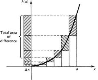
Figure 11.4-3

Using the sum of the kth powers of the consecutive integers from Generalization 2.5-2, we have

which is a polynomial of degree k + 1 in N – 1 (N = the number of rectangles). We rearrange this:

As N goes to infinity, all the terms in the bracket except the first approach zero, and we get the limit,

For the circumscribed sum, we will have one more term in the sum of the kth powers. This approximation produces an N in place of N – 1 in the sum:

but otherwise it is the same. In the limit the result is the same. Thus the circumscribed polygons and inscribed polygons both lead to the same limit (of the two approximate areas):

Looked at in another way (Figure 11.4-4), the difference between the areas of the sums for the circumscribed rectangles and the inscribed rectangles is the single term

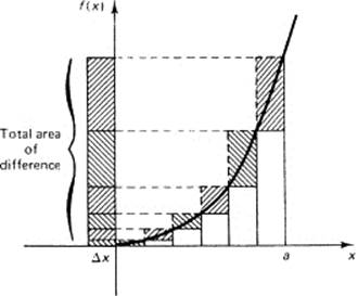
Figure 11.4-4

Therefore, as N approaches infinity, the difference between the circumscribed and inscribed areas must approach 0; both the upper and the lower sums must approach the same limit, and thus they serve to define the area under the curve y – x^k out to x = a. These are often called the Riemann (1826–1866) upper and lower sums.

EXERCISES 11.4

1.Carry out the details for the function y = x³.

2.Carry out the details for the function y = x⁴.

11.5 AREAS IN GENERAL

We now turn to the case of a general function and the area under it (assuming that the function is above the x-axis). Thus we are given a function

y = f(x)

We assume that this is composed of a finite number of pieces each of which is monotone increasing or monotone decreasing (not strictly monotone, but only monotone). See Figure 11.5-1. These are the famous Dirichlet (1805–1859) conditions. Since they permit discontinuities and other reasonable behavior, we are allowing a broad enough class of functions to meet most elementary needs when modeling the real world.

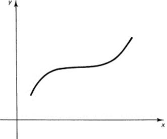
11.5-1 Monotone increasing function

We consider the area under one piece of this function, and argue that if we can find this area then, because the area is additive for any finite number of pieces, we can find the area under the whole function. Suppose we begin at x = a and go to x = b, where a < b. Figure 11.5-2 shows one piece of the function. For convenience, we assume that in this interval f(x) is monotone increasing. The changes for a monotone decreasing function are trivial.

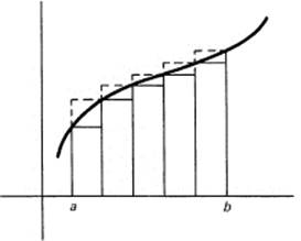
Figure 11.5-2

The difference between the upper sum A_U(N) and the lower sum A_L(N) for equally spaced rectangles will be (Figure 11.5-3 shows these differences projected into a single column on the left)

But

Therefore, the difference between the upper and lower sums is

which must approach zero in the limit as N → ∞. Thus the method of upper and lower sums defines a common limit to associate with the concept of the area under the continuous monotone curve y = f(x) between the two limits aand b.

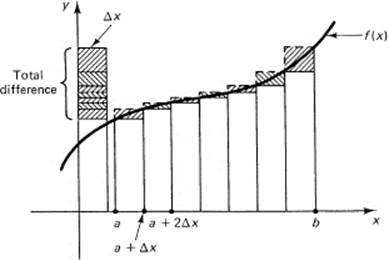
Figure 11.5-3

To generalize the idea of the approximating upper and lower sums of a monotone continuous function, we see first that we need not require that all the rectangles have the same width; they can be of any convenient widths, provided the widest one approaches 0. The projection of all the differences multiplied by their widths onto one column will give a bound:

(see Figure 11.5-4). Thus we have some flexibility in picking the interval widths. Any set of rectangles will do, provided the widest interval approaches 0 in the limit. The difference between the upper and lower sums will be bounded by

The upper and lower sums will therefore approach a common limit, which we call the area under the curve. Further thought shows that the upper and lower sums need not use the same intervals.

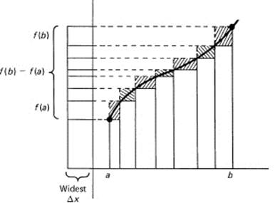
Figure 11.5-4

As a further generalization, we see that we can estimate the sum of the rectangles for a monotone continuous piece of the function by choosing the height of the ith rectangle corresponding to any value θ_i (Greek lowercase theta) of the function in the ith interval:

The estimate for the sum (which in the limit is to approach the area) is now

where the maximum difference x_i – x_i−1 approaches zero in the limit. Hence (Figure 11.5-5), we have for a monotone increasing continuous function

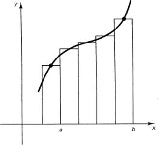
Figure 11.5-5

In mathematical symbols (using the notation of Section 9.9),

For a monotone decreasing function, the inequalities of this last equation are obviously in the opposite direction. Due to the continuity of f(x), the three function values and f(x_i-1), f(θ_i) and f(x_i) all approach the same value in the limit, and hence we see again that the middle sum must also approach the common sum of the two ends as N approaches infinity.

The upper and lower sums are called Riemann sums because he was the first to make general the idea of an area mathematically rigorous. The common limit of the upper and lower sums is called the integral (integrate means to make into a whole). Since his time the concept of an integral has been further generalized, but that development lies beyond the needs of this course.

From the areas of the monotone pieces of the function, we obtain, by simple addition, the area under the whole curve (consisting of a finite number of the pieces of monotone continuous functions).

Thus we see that the limit of the sum can be defined using any arbitrary intervals (as long as the largest approaches 0 as N approaches infinity), and we can pick any typical value in the ith interval as the height of the corresponding rectangle. We are not limited to equal spacing and picking particular values in each interval, nor must the intervals chosen for the upper and lower sums be exactly the same.

Further thinking about what we have done shows that actually we are computing the limit of a sum; the word “area” was only a colorful way of referring to the problem. Integration is actually the computation of the limit of a sum that is chosen in a rather flexible manner; it is not the rigid thing we began with. This is very typical in mathematics; an idea that arises in a specific context is gradually generalized until the original idea is merely a very special case.

We assumed that the two limits between which we were computing the area were different. It is a natural extension of the idea of area (and the generalizations we have made from it) to say that if

b = a then the integral (area) = 0

A further extension is that if b < a then the integral (the limit of the sum) is to be negative, since the Δx_i will be negative. Similarly, if the function is below the x-axis and the Δx_i is positive, we would naturally call the integral negative. Finally, it follows that if b < a and f(x) < 0 then the integral would again be positive, since it would be the limit of a sum of positive terms.

Notice that we began by claiming that area was measured by a positive number or 0, and now we are admitting negative areas. The contradiction is only apparent; we still feel that areas are nonnegative but that at times it is convenient to call an area negative. We made the positive area convention when we first examined areas. Now, due to the generalizations we have made, from our original idea of area to the idea of a limit of a sum, it is convenient to allow negative areas; otherwise, we would be forced to limit ourselves to functions that were nonnegative and sums where b ≥ a. We could easily fix up the contradiction if we wished, but that would later force us into a lot of circumlocutions when we wanted to discuss problems where the areas (sums) cancel. We have only to keep in mind the apparent contradiction and watch for any foolishness that may emerge when we are careless. In a sense, we have extended the idea of area, and this generalization needs to be watched to see all the consequences.

We now introduce the usual notation. The limit of the sum is suggested by the elongated S (Sum) that begins the symbol. The letters a and b at the bottom and top of this elongated S are the limits of the range we are using. The next piece is the name of the function f(x). Finally, we have the name of the variable with respect to which we are summing, the differential dx. We write it in the differential form as

This is called the integral from a to b of the function f(x) with respect to the variable x. In words, “the integral from a to b of f(x) dx.”

The integral can be thought of as an operator, like d/dx, but in the form

where the … is the place for the name of the function to be integrated with respect to the variable x.

If b lies between a and c, then it is clear that (see Figure 11.5-6)

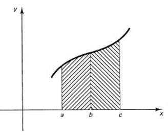
Figure 11.5-6

This is merely the statement that adjacent nonoverlapping intervals add properly for sums as well as for areas. Due to our use of the algebraic sign of areas, it is still true when b is not between a and c (provided the integrals exist). With all this formal apparatus, we can now find sums and areas by a uniform method, rather than a collection of artificial special techniques.

We remind you again, we generalized our primitive ideas about areas until we found that a suitable limit of a sum is the integral of the function. Areas are only a special application of the idea of an integral.

11.6 THE FUNDAMENTAL THEOREM OF THE CALCULUS

The great discovery that made the calculus a “calculus” (a routine process) is that it is sensible to ask, “What is the derivative of the integral?” We now think of the area under a function y = y (x) (or any of the extensions of this idea) as depending on the upper limit of the range of the integration (set b = x):

Before going on, it is convenient to remove a possible source of confusion. The x in the above integrand is a dummy variable in the sense that if we used any other letter for the variable x, say the letter t in

f(x)dx

then in its place we would have

f(t)dt

and we would have the integral

The area (or, more generally, the limit of the sum) would be the same. The reason is simply that the expression says that the variable of summation goes from the lower limit of integration a to the upper limit x. This change of the dummy variable of integration is exactly the same as we have for summation:

Whether we use n or m makes no difference in the answer. If we do not make this change in notation for the integral (11.6-1), we will become confused with the different meanings of x. In the old form it was both the variable of summation and the value we used as the upper limit in the final sum. In the new form we are summing and then taking the limit of a set of function values times the corresponding interval widths, depending on the dummy variable t, and using x as the upper value.

We now ask, “What is the derivative of this integral?” What is

Intuitively, what are we asking? For a continuous curve f(x), when f(x) is a large number, the area is increasing rapidly, and where f(x) is small, the area is increasing slowly. The rate of growth of the area under a continuous curve is exactly the height of the curve at that point.

Due to the importance of this result, we need to back up our intuition with some rigor; in the past we have occasionally found that our intuition led us astray.

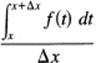
The question of what is the derivative with respect to the upper limit of the integral is a basic question, and we therefore go back to the basic definition of a derivative, the four-step process of Section 7.5. At step 4 we are to take the limit of the difference quotient:

But since this is the difference between two partially overlapping ranges of integration (Figure 11.6-1), the result must be merely over the range that is not common to both, that is, x to x + Δx. (Remember that Δx can be either positive or negative.) Therefore, we have

If we think of f(t) as being a positive, continuous, monotone increasing function in this interval (decreasing makes trivial changes), then (going back to the sum definition of the integral) we have the bounds on the function in the interval Δx. If Δx is positive, then

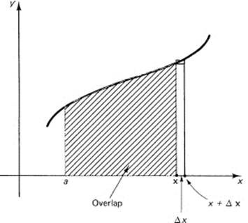
Figure 11.6-1

lower bound = f(x) and upper bound = f(x +Δx)

where Δx is the length of the integration interval. Because f(x) is continuous, as Δx approaches 0 we have the same upper and lower bounds. And similarly for Δx negative. Thus we conclude that the derivative of the integral with respect to the upper limit of integration x is simply the function being integrated, the integrand. Be sure you see the inevitability of this result. Think about what is happening as the derivative of the integral is taken, how the rate of growth of the area under a continuous curve must be exactly the height of the curve at that point. The mathematics this time matches our intuition.

This is the fundamental theorem of the calculus,

(where a is some fixed value of x); the derivative with respect to the upper limit of the integral of a function is the function itself. Thus differentiation undoes integration. We see the truth of this in the integration of x^k, Generalization 11.4-3. The integral with the upper limit x [use x in place of a in the formula (11.4-4)] is

Differentiating this with respect to x, we get the original integrand,

as the theorem requires. Thus integration is the inverse operation to differentiation, just as division is the inverse to multiplication. In both cases (division and integration), it comes down to a guess process. The question in integration is, “What function is this the derivative of?”

While the derivative of the integral is the original function, it is not true in general that the integral of the derivative of a function is the original function (the two operations do not “commute”). The reason for this is simple. Consider two functions that differ by a constant. Since the derivative of a constant is zero, their derivatives are the same. Therefore, given only the derivative, we cannot know which one was the original function. We know the integral only to within an additive constant; there is an arbitrary additive constant to be tacked onto the integration process when we think of integration as the antiderivative.

Example 11.6-1

Given that the derivative of a polynomial is

we find that the antidervative is (where C is some constant)

After some algebra, this is simply

You can always check an integration by differentiating the answer to recover the original expression.

Thinking about the matter (upper and lower sums, the limit, and the continuity in each interval), we see that the sum of two functions added together is the same as the sum of the two individual sums added together; integration is a linear operator, just as differentiation was.

We also see from the fundamental theorem of the calculus that since we can differentiate any powers, not only integral powers, we can also integrate them. It is convenient to write the formula for integration in terms of the antiderivative (any function whose derivative is the given function) of a single power of x as

for any n other than n = –1. We have deliberately omitted the limits of integration for the antiderivative, and have supplied the missing constant C that is arbitrary when we handle the antiderivative.

We clearly cannot do the case n = –1 using this formula, both because it requires a division by zero and because no differentiation of a power of x leads to the exponent –1. We will take up the problem of its integration in Chapter 14.

We need some notation. It is very convenient to write an antiderivative of f(x) as F(x). We have, therefore,

To get from the antiderivative to the integral between the limits of an interval, we merely note that the integral over an interval of no length

so that we must have for the special value x = a

From this we see that

C = −F(a)

or in general

where F(x) is any antiderivative of f(x). Notice how the additive constant C in the antiderivative F(x) disappears in the final result.

It is customary to call the antiderivative the indefinite integral, as contrasted with the integral with limits, which is called the definite integral.

Besides polynomials and sums of arbitrary powers of x (excluding n = –1), we can integrate many different expressions when we recall (Section 7.6) the function of a function formula for differentiation:

Example 11.6-2

What is the antiderivative of

We identify the u of formula (11.6-4) with

u = 1 + x²

Then the du/dx = 2x, and we have the form

which integrates into

It is always easy to check the antiderivative by the simple process of direct differentiation of the answer, and in this case we see that we have the correct antiderivative.

The constant of integration for the indefinite integral is not unique as the following example shows: one C is the other C + .

Example 11.6-3

Given the function to integrate

we can think of it as the sum of two terms and get the answer

or we can think of it in the form

u = x + 1

and get

We see that the letter C is not the same in the two cases.

Let us solve this same problem in the differential notation. We have

dy = (x + 1)dx

Upon integrating both sides, we get

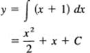
The result is, of course, the same.

The lack of uniqueness of the constant of integration can cause confusion for the beginner when the results obtained are not those in the book.

Example 11.6-4

What is the antiderivative of

We write this in the differential form

Again, how shall we pick the u? The radical is awkward, so we pick

u² = 1 – x²

because this form will get rid of the radical. we get

We now have

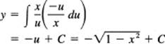
Differentiation confirms this result.