Methods of Mathematics Applied to Calculus, Probability, and Statistics (1985)
Part I. ALGEBRA AND ANALYTIC GEOMETRY
Chapter 3. Fractions—Rational Numbers
3.1 RATIONAL NUMBERS
In school, after studying the integers, you turned to the fractions, which were numbers of the form
![]()
where p and q are integers, and q ≠ 0.
Unfortunately, the word “fraction” has been generalized to include other numerators and denominators than integers. The reason for this is that the rules for handling fractions turn out to include the more general numbers like
![]()
which are often called surds. The name rational numbers (ratio numbers) was introduced to describe the case of one integer divided by another.
A number of conventions are used when handling rational numbers. A proper rational number (fraction) is one whose numerator is less in size than is the denominator. For example,
![]()
is a proper rational number, while
![]()
is an improper rational number. A rational number whose denominator is 1, or whose numerator is 0, is equivalent to an integer. Similarly, rational numbers like
![]()
are equivalent to integers. The integers are, then, special cases of rational numbers. Expressions like
![]()
are integers as well as rational numbers.
There is a natural association of numbers with points on a line (Figure 3.1-1). We pick an endless straight line, mark an arbitrary point as 0, and then place the positive integers 1, 2, 3, …at equal spaces toward the right. The negative integers are placed correspondingly to the left. The fractions then find their appropriate places; for example ![]() is midway between 1 and 2. The line is unending in either direction.
is midway between 1 and 2. The line is unending in either direction.
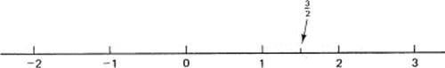
Figure 3.1-1 Numbers arranged on a line
A basic trouble with rational numbers soon arises. For example,
![]()
shows two different representations of the same number. In general
![]()
for any integer k ≠ 0. Thus the same rational number (the same point on the line) has infinitely many different representations. Note that k may be either positive or negative. It is natural to regard the representation with the smallest positive denominator as the lowest, canonical form(canonical means reduced to the simplest form).
We must, therefore, investigate how to reduce a given rational number to its lowest form. The answer is given by applying Euclid’s algorithm to the numerator and denominator to find the greatest common divisor k (see the next section). Once we have the k, we can divide it out of both the numerator and denominator and obtain the lowest form. The word algorithm means an explicitly described process that is certain to end in a finite number of steps.
3.2 EUCLID’S ALGORITHM
Euclid’s algorithm finds the greatest common divisor (the largest factor common to both) of two integers, say p and q. This is often abbreviated as GCD (greatest common divisor). If we suppose thatp is larger than q (and both are positive for convenience), the plan is to divide p by q to get a quotient and a remainder. We will then divide the q by this remainder, getting another quotient and remainder, and repeat this process an indefinite number of times.
We have a problem of notation. Let us relabel the first number p as r0 and the second number q as r1, with r0 larger than r1. We divide r1 into r0 to get the quotient q1 and a remainder r2; that is,
![]()
or, as mathematicians prefer to write the equation,
r0 = q1r1 + r2
where, of course, the remainder r2 is less than the divisor r1. Note that any number that divides both r0 and r1 must also divide r2 (since a fraction cannot be equal to an integer, and q1 is an integer). Since we have reduced the size of one of the numbers, we next divide r1 by r2 to get a new quotient q2 and a new remainder r3.
r1 = q2r2 + r3
Again, any number dividing r1 and r2 must also divide r3. We can repeat this process until we get a remainder of 0. This must happen, because at each step we are reducing the size of the (integer) remainder and therefore we must ultimately reach 0.
We write out all the equations in a single block so we can inspect them. Let rn+1 be the zero remainder. We have
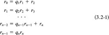
Any number that divides both r0 and rx must finally divide rn. But rn might have other factors, and hence we must investigate this.
We see from the bottom line that rn divides rn–1. Looking at the next equation up the array, we see that since rn divides both itself and rn–1 it must also divide rn–2. And so on up to the statement that rn divides r1 and therefore from the top line must divide r0. Thus rn divides both r0 and rx, and r1 is the greatest common divisor (GCD) of both of the original numbers r0 and rx, which is what the algorithm is designed to produce.
Example 3.2-1
It is often wise to try out a general formula on a few special cases. Take the integers 24 and 18. The set of equations (3.2-1) becomes
24 = 1(18) + 6
18 = 3(6) + 0
and we see that 6 is the greatest common divisor of 24 and 18. Next, suppose the starting numbers are relatively prime (have no common factor), for example 32 and 27. We have, corresponding to (3.2-1),
32 = 1(27) + 5
27 = 5(5) + 2
5 = 2(2) + 1
2 = 2(1) + 0
The last line is trivial and is not worth the effort. Once a remainder of 1 occurs you know there is no common factor except the trivial factor 1.
This algorithm is included for a number of reasons: to solve the problem of reducing a rational number to its lowest form; to illustrate the concept of an algorithm, which is a central idea in mathematics and computing; and for several other purposes, which will emerge later (Abstraction 4.6-1; multiple zeros, Section 9.8; and partial fractions, Sections 17.2 and 17.3). An algorithm is a definite process that is known to terminate in a finite number of steps. Especially in the field of computer programs, the algorithm must be exactly described for all the possibilities that can arise and must be shown to terminate in a finite number of steps.
EXERCISES 3.2
1.Find the GCD of 12 and 28.
2.Find the GCD of 22 and 39.
3.Find the GCD of 287 and 343.
4.Find the GCD of 256 and 243.
5.Was it necessary to assume that the first number r0 was larger than the second, r1? What would happen if it were not?
6.How would you handle negative numbers in Euclid’s algorithm?
3.3 THE RATIONAL NUMBER SYSTEM
When we consider the rational numbers, we find that there are a couple of surprises in store. First, unlike the integers, there is no next number along the line on which they are conventionally placed, because between any two distinct rational numbers we can place as many more numbers, equally spaced or otherwise, as we please. We have only to take the difference between the two given numbers, break it into N equally spaced intervals each of length 1/N times the difference, and then repeatedly add this length onto the starting number. These N – 1 numbers will fall between the given two rational numbers. Generally, these interpolated numbers will be fractions, but some of them could be integers.
Example 3.3-1
Interpolation of n numbers between two given numbers. Suppose ![]() and
and ![]() are the given numbers, and we want to insert 10 numbers between them. We therefore need 11 intervals, N = 11. The arithmetic is
are the given numbers, and we want to insert 10 numbers between them. We therefore need 11 intervals, N = 11. The arithmetic is
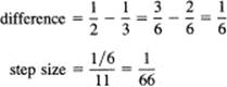
The 10 desired numbers are, therefore,
![]()
The next number,
![]()
is the other end number. This is a convenient check on the arithmetic.
We see that the rational numbers are everywhere dense along the line, meaning just what we proved: no matter how finely spaced you think the numbers are, there are as many more numbers in any given interval as you please—and even more than that! Furthermore, in some sense, the numbers are uniformly dense on the line; no interval of the line has more rational numbers than any other interval of the same length or any other length. Figure 3.3-1shows that in some sense each point on the short segment corresponds uniquely to a point on the long line segment.
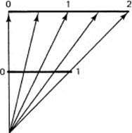
Figure 3.3-1 The interval [0,1] mapped onto [0, 2]
The rational numbers have the further property that any additions, subtractions, multiplications, or divisions (other than by 0) can be done and the answer is another rational number. This property of the rational numbers is called closed with respect to the operations mentioned. As far as these four operations are concerned there are no gaps in the rational number system; no need for further numbers can arise within the system.
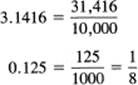
All decimals that have only a finite number of nonzero digits (with all 0’s past some point if you wish) are clearly rational numbers whose denominators are suitable powers of 10. For example,
Similarly, the integers are closed with respect to the three operations of addition, subtraction, and multiplication. It is the operation of division that forces us to consider the rational numbers.
EXERCISES 3.3
1.What would happen in Example (3.3-1) if the ends of the interval were reversed?
2.Insert 7 numbers between ![]() and
and ![]() .
.
3.Describe all numbers having a terminating decimal number representation.
4.Describe all numbers having a terminating binary (base 2 instead of 10) representation.
5.Write the formulas for interpolating N numbers between a and b.
3.4 IRRATIONAL NUMBERS
We return to Pythagoras again. It is often claimed that he (or one of the Pythagorean sect) first discovered that the square root of 2 is not a fraction. The proof probably went somewhat as follows and arose from the problem of the length of the diagonal of a square of unit size (Figure 3.4-1).
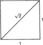
Figure 3.4-1 The diagonal of a unit square
Example 3.4-1
The ![]() is an irrational number. We want to prove that
is an irrational number. We want to prove that ![]() is not a fraction p/q. Most impossibility problems begin by assuming that the opposite is true and then produce a contradiction, thus showing that the assumption is false and hence that the representation is impossible. Therefore, we suppose, contrary to what we wish to prove, that the
is not a fraction p/q. Most impossibility problems begin by assuming that the opposite is true and then produce a contradiction, thus showing that the assumption is false and hence that the representation is impossible. Therefore, we suppose, contrary to what we wish to prove, that the ![]() is a rational number; that is,
is a rational number; that is,
![]()
and the fraction p/q is in its lowest (canonical) form (p and q have no common factors). To get rid of the new operation (the square root), we square both sides of (3.4-1) (what else could we do?). Thus we get
![]()
Cleared of fractions,
![]()
The left side is clearly an even integer.
Every odd integer is of the form 2k + 1 (for some integer k), and the square of the odd integer 2k + 1 is
(2k + 1)2 = 4k2 + 4k + 1
which is again an odd integer. It follows that p could not be an odd number; it must be an even integer. Therefore, let
p = 2m
and put this into Equation (3.4-2):
2 q2 = 4m2
Dividing out the 2, we have
q2 = 2m2
A similar argument shows that q is also even. We started with the fraction in lowest form and have found a contradiction, since 2 divides both p and q. Mathematics generally insists on no contradictions, so we look back to find the suppose and decide that what immediately follows must be false.
Since we have just shown that ![]() is not a ratio number, it is therefore called an irrational number (not a ratio number).
is not a ratio number, it is therefore called an irrational number (not a ratio number).
Generalization 3.4-2
Irrational numbers in general. A far more direct, and more general, proof of the irrationality of various roots is based on the simple observation that when you take a fraction (that is not an integer) and square it you will not get an integer, because the denominator cannot completely cancel out. Therefore, you can see that for all square roots, indeed for all cube roots, fourth roots, and so on, if the root is not an integer, then it cannot be a fraction.
The irrationality of ![]() certainly came as a surprise to the ancient Greeks. The rational numbers are everywhere dense along the line, yet
certainly came as a surprise to the ancient Greeks. The rational numbers are everywhere dense along the line, yet ![]() is not one of them! In The Elements, Euclid effectively decided that
is not one of them! In The Elements, Euclid effectively decided that ![]() was a magnitude but not a number. Eudoxus had already (around 360 B.C.) created an elaborate theory to handle magnitudes. We, on the other hand, have decided that there should be a number that measures the diagonal of a unit square, that is, V2. See Figure 3.4-1. Similarly, for other such lengths that are not represented by rational numbers, we feel that there should be a number that measures the length. To get a deeper look at this apparent paradox that the everywhere dense rational numbers do not exhaust the points on the line, we look at the decimal representations of irrational and rational numbers in the next two sections.
was a magnitude but not a number. Eudoxus had already (around 360 B.C.) created an elaborate theory to handle magnitudes. We, on the other hand, have decided that there should be a number that measures the diagonal of a unit square, that is, V2. See Figure 3.4-1. Similarly, for other such lengths that are not represented by rational numbers, we feel that there should be a number that measures the length. To get a deeper look at this apparent paradox that the everywhere dense rational numbers do not exhaust the points on the line, we look at the decimal representations of irrational and rational numbers in the next two sections.
EXERCISES 3.4
1.Define an irrational number.
2.Prove that ![]() ≠ p/q using the method of Example 3.4-1.
≠ p/q using the method of Example 3.4-1.
3.Same for ![]() .
.
4.Prove that ![]() is irrational.
is irrational.
5.Why does the proof fail for ![]() ? At what step does this occur?
? At what step does this occur?
6.Prove that, if the polynomial with integer coefficients
![]()
has a root that is an integer, then the root divides a0.
7.*Prove that, if the polynomial with integer coefficients
![]()
has a rational root p/q, then p divides a0 and q divides an.
3.5 ON FINDING IRRATIONAL NUMBERS
We now investigate these irrational numbers, in particular, how to find their decimal representations.
Example 3.5-1
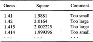
An algorithm for finding some irrational numbers. How might we find the decimal representation of ![]() ? The only property of the number we know is that its square is the number 2. Let us use this. We make a first guess that the square root is 1. We observe that the square of 1 is 1 and that this is too small. This suggests that we try the number 2 as the next guess, and we find that 2 squared is 4, which is too large. We suspect that a better guess would be around 1.5. The square of 1.5 is 2.25, which is too large by a small amount. So we try 1.4 whose square is 1.96, a bit too small.
? The only property of the number we know is that its square is the number 2. Let us use this. We make a first guess that the square root is 1. We observe that the square of 1 is 1 and that this is too small. This suggests that we try the number 2 as the next guess, and we find that 2 squared is 4, which is too large. We suspect that a better guess would be around 1.5. The square of 1.5 is 2.25, which is too large by a small amount. So we try 1.4 whose square is 1.96, a bit too small.
We see that there exists an organized method of search for better and better approximations to ![]() . At each stage of the process we try a reasonable guess between a number known to be too large and one known to be too small. By this method we can come as close as we please to the square root of any positive number.
. At each stage of the process we try a reasonable guess between a number known to be too large and one known to be too small. By this method we can come as close as we please to the square root of any positive number.
We continue the search method to be sure you understand it. Since 1.96 is much closer to 2 than is 2.25, we first try 1.41.
We see that we have a recursive process that can improve any approximation we have at hand; we merely interpolate a good guess between the current known upper and lower bounds and thus get an improved bound on one side or the other. The process will never end for the square root of 2, since we know that the number we are approximating is an irrational number, and every terminating decimal is clearly a rational number (since it is an integer divided by some power of 10). We are not, at present, interested in an efficient search method, although we will be later (Section 9.7). Our interest is in the concept of recursively finding better and better approximations to a number when we are given a property that suitably defines the number. This is an algorithm, provided we agree to stop at some preassigned level of accuracy.
Example 3.5-2
Suppose we want to find the numerical value of the positive zero of the equation
x2 – x – 1 = 0
Consider the left-hand side as a function of x; that is, write
f(x) = x2 – x – 1
For x = 1 we get the value – 1; for x = 2 we get the value +1; hence the value of x we want (which makes the left-hand side zero) lies between 1 and 2. Since the two polynomial values are equal in size and opposite in sign we naturally guess that the true value lies near 1.5. We get from the left-hand side of the equation the corresponding value –0.25, so we need a slightly larger value. Let us try 1.6. By now we need to tabulate things:
|
x value |
Polynomial value |
|
1.6 |
−0.04 |
|
1.7 |
0.19 |
|
1.62 |
0.0044 |
|
1.61 |
−0.0179 |
|
1.618 |
−0.000076 |
|
1.6181 |
0.00014761 |
And so on. This process can find as many decimal places as you desire, provided you are willing to do all the arithmetic. The actual number is the golden ratio of Section 2.4:
![]()
as can be seen from the formula for the roots of a quadratic (if you remember it, and if you do not remember the formula, then see Example 6.3-2).
Generalization 3.5-3
Finding zeros of simple (smooth) equations. This method of finding the decimal expansion of a number from its defining equation by using successive approximations, in the above cases x2 – 2 = 0 and x2 – x – 1 = 0, can be applied to many (but not all) numbers. We simply use the defining equation, and by noting the sign of the value of the corresponding function we generate a new estimate of the number. By sufficient work we can reduce the size of the interval in which a sign change occurs to be as small as we please. Thus we have a bound on the accuracy of the result, one number is smaller and one number is larger than the sought for root of the equation, and they are as close together as you wish (and are willing to compute).
The central problem in finding the representation of a number is to find an equation of which it is a solution. This is a matter of inspiration in the general case, but often it is fairly easy to do. Once we have its defining equation, we are on the path to its representation (in any number base we wish).
EXERCISES 3.5
Using three-decimal arithmetic, do the following problems.
1.Find ![]() .
.
2.Find ![]() .
.
3.Find ![]() .
.
4.Find ![]() .
.
5.Find the real zero of 9x3 + 9x2 + 3x – 1 = 0
6.Find the real root of x3 + 7x2 + x – 4 = 0.4.
7.Find the positive zero of Newton’s cubic x3 – 2x – 5. Ans.: 2.0945 ….
8.Find the two positive roots of x3 – 3x + 1 = 0.
9.When using a computing machine, it is customary to bisect the interval at each stage rather than try to interpolate a next guess. Show that for every ten iterations of this bisection method you gain at least three decimal digits in accuracy.
10.*Describe the bisection method in some detail, including the starting assumptions. Note that you must allow for hitting the zero in the middle of the process. Apply to ![]() to three decimal places.
to three decimal places.
3.6 DECIMAL REPRESENTATION OF A RATIONAL NUMBER
To find the decimal form of a rational number, we merely divide the numerator by the denominator.
Example 3.6-1
When the number ![]() is divided out, we get
is divided out, we get
![]()
where the ellipsis dots mean an unending string of 3’s, and the bar over the 3 means repeat endlessly. This decimal representation is periodic with a period of one decimal digit, 3. If we try ![]() , we get
, we get
![]()
By filling in the endless string of 0’s, we write a comparable form to the endless string of 3’s. Again we have a period of one.
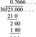
Next consider a rational number like ![]() . Here we need to explicitly divide it out:
. Here we need to explicitly divide it out:
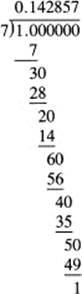
and we see that the remainder 1 will start the same period again. Thus
![]()
where this time the ellipsis means the endless repetition of the block of six digits, 142857.
A little study will convince you that once you have passed beyond all the digits of the numerator and begin the “bringing down of the zeros” then the periodicity is inevitable. Each remainder is less than the divisor, and therefore in not more steps than the size of the divisor the same remainder must occur again. (For the denominator q there cannot be q consecutive remainders without a duplicate or else a 0. A zero remainder, of course, produces all zeros after this point and has a period of one.) Thus we see that rational numbers must have periodic decimal expansions, once we get past a finite number of leading digits, which may be almost anything depending on the numerator. But the numerator being a finite number can affect only a finite number of places, and then the “bringing down of the zeros” begins.
Example 3.6-2
As a very simple example of the effect of nonzero digits in the numerator, consider the fraction
![]()
Divide this out to get
Hence
![]()
We next ask the converse: Is a periodic decimal number always a rational fraction? To answer this question, we need to look closer at the meaning of a decimal number. The number 0.333 … is defined to be the expression
![]()
For a finite number of terms, this resembles the geometric progression
a + ar + ar + … + arn–1
of Example 2.6-1 with a = ![]() and the rate r =
and the rate r = ![]() . If we take only the first n digits of the decimal expansion, then the sum is, according to the formula for a geometric progression (2.6-1),
. If we take only the first n digits of the decimal expansion, then the sum is, according to the formula for a geometric progression (2.6-1),
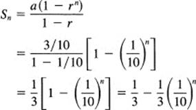
But the term (![]() )n approaches zero as n gets large. Hence as n gets larger and larger the numerical value of the number represented by the first n digits gets closer and closer to the first term, which is
)n approaches zero as n gets large. Hence as n gets larger and larger the numerical value of the number represented by the first n digits gets closer and closer to the first term, which is
![]()
If you believe that there is a difference between the endless string of 3’s and the fraction ![]() , then when you state this (nonzero) size, no matter how small a number you choose, it is clear that I can tell you how far out to go along the endless string of 3’s so that you will then get and remain closer (if you go still farther) than you required. Therefore, there is a contradiction with your assumption that you could name a difference. The difference between
, then when you state this (nonzero) size, no matter how small a number you choose, it is clear that I can tell you how far out to go along the endless string of 3’s so that you will then get and remain closer (if you go still farther) than you required. Therefore, there is a contradiction with your assumption that you could name a difference. The difference between ![]() and the n digit terminated decimal number becomes arbitrarily small as n becomes large. Thus one is inclined to say that there is no difference between the number represented by the infinite (endless) decimal expansion 0.3333 … and the number
and the n digit terminated decimal number becomes arbitrarily small as n becomes large. Thus one is inclined to say that there is no difference between the number represented by the infinite (endless) decimal expansion 0.3333 … and the number ![]() .
.
We can also go back to the fundamental “trick” for summing a geometric progression and use it directly to shorten the argument. Let
x = 0.333333 …
then
10x = 3.33333 …
Subtract the upper from the lower expression (it is not exactly clear how you can do this for the infinitely long string of digits but it seems “reasonable” that the difference is 3):
10x – x = 3
We now solve for x
9x = 3
x = ![]()
Example 3.6-3
We may apply the same method to any repeating decimal. For example, let
x = 4.6373737 … = 4.63 7
The period for repetition (37) is two digits, so we write
100x = 463.737 …
and subtract from this the original value
(100 – 1)x = 463.73 7 – 4.63 7 = 459.1
from which we get
![]()
Direct division will produce the original string of digits.
Example 3.6-4
If we apply this same reasoning to the decimal expansion
x = 0.9999 … = 0.9
and if we use the geometric progression argument, then we have a = ![]() and r =
and r = ![]() . The formula for the sum of the finite geometric progressin involving only the first n digits is
. The formula for the sum of the finite geometric progressin involving only the first n digits is
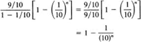
Again, as n becomes larger and larger, the rn term rapidly approaches zero. Thus a string of endless 9’s appears to be the number 1. After all, there can be no numerical difference between the two represented numbers, 0.9999 … and 1, no matter how small you think the difference is. Hence we conclude that they are just different representations of the same number.
If we use the short version, we get
10x = 9.99 …
and on subtracting the original expression we get
9x = 9
x = 1
as before.
Generalization 3.6-5
If the preceding example seems strange, it merely means that some numbers may have two different appearing decimal representations. A number like
2.3459999 …
where the three dots mean all 9’s, may also be written as
2.3460000 …
Calling the two different representations the same number is convenient because there is no difference in their numerical values. If you think that there is, then (for yet one more time) it is easy to show that, no matter how small you think the difference is, the sequence of digits can be pushed until the difference is less than you claimed. Hence your “if” must be wrong.
To summarize where we are, we have found that the rational numbers have periodic decimal expansions (and by extension this is true for any other integer base, including base 2). Conversely, periodic decimal expansions (or for any other integer base) correspond to rational numbers. The irrational numbers, therefore, cannot have periodic decimal expansions. Conversely, nonperiodic decimal expansions correspond to irrational numbers.
This is an explanation of how there can be numbers other than the everywhere dense rationals—all those numbers whose decimal expansions do not end with a periodic structure are not rational numbers; they are by definition the irrational numbers. Periodicity in the decimal expansion of a number is a very great restriction; once past the nonperiodic part, every digit is determined by the periodicity. For other numbers the digits are not so restricted, so apparently the nonperiodic expansions are, in some sense, much more numerous. But recall Galileo’s observation that in a certain sense the integers and their squares are equally numerous (Section 2.1). We are not in a position to prove that the irrational numbers are very much more numerous than the rationals; we are reduced to stating the fact and indicating loosely why this might be so.
Along the way we have seen enough special cases of a geometric progression with the rate r less than 1 in size to realize that it is reasonable to say that the infinite series of terms has the sum
![]()
A more careful proof of this will be given in Section 7.2.
EXERCISES 3.6
1.Find the decimal representation of ![]() .
.
2.Find the decimal representation of ![]() and the period.
and the period.
3.Find the fraction equivalent to 0.121212 ….
4.Find the fraction equivalent to 3.145145 ….
5.Find the fraction equivalent to 1.51515 ….
6.Find the fraction equivalent to 0.0011111 ….
7.Show that adding the corresponding decimal fractions agrees with the equation ![]() +
+ ![]() =
= ![]() . How about
. How about ![]() +
+ ![]() =
= ![]() ?
?
8.Write out the details for finding the binary representation of a decimal number less than 1.
9.Show that jo in binary notation has an endless periodic representation, and hence that ![]() +
+ ![]() + … +
+ … + ![]() (ten times) when rounded off to a fixed number of binary places will not total up to 1.
(ten times) when rounded off to a fixed number of binary places will not total up to 1.
10.An ideal bouncing ball rebounds each time to a height k (less than 1) times the height it fell from on that bounce. If the initial height is h, find the total distance the ball travels.
3.7 INEQUALITIES
When dealing with integers, there is a “next number,” but when dealing with the rational numbers, which are everywhere dense, there is not a “next number” (since, for example, the average of two numbers lies between them). The irrational numbers have the same property that there is no “next number.” In place of “next” we introduce the ordering of the numbers by the use of the inequality. For the moment, think of a and b as rational numbers.
a < b
means a is less than b, that a lies to the left of b on the line that we conventionally use to represent the values of numbers. For example,
7 < 8
and for negative numbers
–8 < –7
We also write these as
8 > 7 and –7 > –8
(8 is greater than 7). In both cases the pointed end of the symbol points to the smaller number. It is often convenient to say “greater than or equal to” which in mathematical notation takes the form
8 ≥ 7
In general symbols we have both
a ≤ b and b ≥ a
as the same inequality.
We can add inequalities in the same sense. For example, if
a ≥ b and c ≥ d
then
a + c ≥ b + d
A slightly more mathematical proof of this can be given. The inequality
a ≥ b
means
a – b ≥ 0
Similarly,
c – d ≥ 0
The sum of two positive numbers is positive, so we have
a + c – b – d ≥ 0
and then we have the result when we transpose the two negative terms.
We cannot subtract inequalities, as you can see from making up simple examples. Of course, the same number can be subtracted from both sides of an inequality.
We can multiply both sides of an inequality by the same positive number and retain the inequality. For example,
6 < 7
becomes, when multiplied by 3,
18 < 21
But if we multiply by a negative number, then the sense of the inequality is reversed. In the same example, multiplying by –3 produces
–18 > –21
In mathematical symbols, if a ≥ b and c ≥ 0, then, using the fact that the product of two positive numbers is positive, we have
(a – b)c ≥ 0
ac – bc ≥ 0
from which it follows that
ac ≥ bc
Multiplication by a negative number is easily seen from the above to reverse the inequality.
We can also take the positive square roots of quantities greater than 0 and maintain inequalities. To prove this we need to show that if
0 < a < b
then
0 < ![]() <
< ![]()
One method of proof is to assume that the opposite is true, that
![]() ≤
≤ ![]()
Then multiplying each term by the positive number ![]() will give
will give
0 > ![]()
![]() ≤
≤ ![]()
![]() ≤
≤ ![]()
![]()
where we have used the assumption that ![]() ≤
≤ ![]() in the last step. From this we have
in the last step. From this we have
0 < b ≤ a
which is an immediate contradiction.
Example 3.7-1
An important inequality. We will use these ideas to prove the important inequality that if a > 0 then
(1 + a)n ≥ 1 + na
when n is an integer and n ≤ 1. The proof is by induction. For the case n = 1 it is clearly true (indeed the case n = 0 would also serve). We therefore assume it is true for the case m – 1; that is, we assume
(1 + a)m–1 ≥ 1 + (m – 1)a
with m ≥ 2. To get to the next case we must, for this induction, multiply both sides by the positive number 1 + a. We get
(1 + a)m ≥ [1 + (m – 1)a] + [a + (m – 1)a2]
If we drop the nonnegative number (m – 1)a2 from the right-hand side, we can only strengthen the inequality. The result is
(1 + a)m ≥ 1 + ma – a + a = 1 + ma
as required for the induction process.
We could also have proved the inequality by using the binomial theorem expansion
![]()
and dropping all the positive terms after the first two terms. Remember that a > 0.
This shows that often the same result can be found in different ways. Since we are concerned with methods, we shall often find the same result by several different methods. One advantage of alternative proofs is that when we “listen to the mathematics” involved in the proofs we can then learn different things about the same result. Furthermore, when we come to extend, or generalize, a formula, one derivation may be more appropriate than another.
EXERCISES 3.7
Hint: Try specific numbers first before discussing the general case. Be sure to try positive, zero, and negative numbers.
1.Under what conditions can inequalities be multiplied term by term?
2.Under what conditions can inequalities be divided term by term?
3.Show that 1 < ![]() <
< ![]() < 2.
< 2.
4.Prove that 2xy ≤ x2 + y2.
5.*Schwartz Inequality: In Exercise 4 set xi = ai/{a12 + a22 + … + an2}1/2 and yi = bi/{b12 + b22 + … + bn2}1/2. Apply the result of Exerciese 4. Then add for all i to get x1y1 + x2y2 + … + xnxn ≤ 1. Finally, rewrite in terms of aiand bi to get
a1b1 + … + anbn ≤ [a12 + … + an2]1/2[b12 + … + bn2]1/2
3.8 EXPONENTS—AN APPLICATION OF RATIONAL NUMBERS
We have already used some simple properties of exponents with which you are familiar. We are reviewing the topic in more detail to provide a pattern of abstraction and generalization that we will often refer to. Thus it is the methods (as well as the results) that require your attention.
Example 3.8-1
The laws of exponents are a good example of simply listening to what a formula says. Descartes (1596–1650) popularized the compact notation for writing a sequence of copies of the same symbol (notice we are not asserting that a is a number):
![]()
where there are n symbols a on the left. Just reading what the following symbols mean (m copies of the symbol a followed by n copies), it is clear that
![]()
Similarly,
![]()
We are clearly using the ellipsis method of proof. The more formal method of mathematical induction can be used if you wish, but it hardly makes things more convincing.
Extension 3.8-2
To extend the concept of exponents to the integer 0, we simply put n = 0 in Equation (3.8-2) to get
am a0 = am
from which clearly (assuming, of course, that a ≠ 0)
![]()
(where the symbol “1” is the identity if you think that a is a general symbol, and is the number 1 if you think of a as a number). We get a consistent result from (3.8-3) when m = 0. Thus this seems to be a reasonable extension of the meaning of an exponent.
The next extension of the idea is to negative exponents. We do this by setting n = –m in Equation (3.8-2):
![]()
from which it follows that (dividing by am)
![]()
We next extend the idea of exponents to the rational numbers. This was first done by Nicole Oresme (1323–1382). What could
a1/2
possibly mean? Again using Equation (3.8-2) with m = n = ![]() , we have
, we have
a1/2a1/2 = a1 = a
Alternately, from Equation (3.8-3),
(a1/2)2 = a1 = a
These equations both ask, “What symbol multiplied by itself gives oT The answer (when adjacency of the symbols means multiplication of numbers) is, of course, the square root of a; that is,
![]()
(always supposing that the root exists). It follows from a similar argument (it is supposed that you can now supply the details for this simple extension) that
![]()
Furthermore, since
![]()
it follows that
ap/q = (qth root of a)p
It takes only a little thinking of what you mean by the qih root of a product to convince yourself that, for positive numbers,
the qth root of a product is the product of the qth roots
(abc …)1/q = a1/q b1/q c1/q …
We have only to multiply the right-hand side by itself q times and regroup the letters (assuming that the symbols commute with one another) to see the truth of this statement.
For negative numbers, you must do some careful thinking first before using the laws of exponents freely. Odd-order roots of a negative number are negative, while even-order roots are imaginary (see Section 4.8).
It was necessary to convince ourselves that the equality of the symbols
![]()
when viewed as rational numbers is also true when they are used as exponents. The formal writing of the symbol is not enough; you must verify that the extension is valid in all the properties you use.
EXERCISES 3.8
1.Evaluate (a) x7x6; (b) x7x6; (c) (x7)6.
2.Evaluate (a) x3/2xl/2; (b) x–3x–4; (c) x–(2/3)x–(1/2).
3.Show that ![]()
![]()
![]() = 6.
= 6.
4.Show that (![]() )5 = 4
)5 = 4![]() .
.
5.Show that (![]() /2) = 1/
/2) = 1/![]() .
.
6.Show that a/![]() =
= ![]() .
.
7.Show that (![]() /2)(
/2)(![]() /2)(
/2)(![]() /2) =
/2) = ![]() /4.
/4.
8.Show that ![]() .
.
9.Show that [(ab)c]d = [(ad)c]b
3.9 SUMMARY AND FURTHER REMARKS
This chapter examined a few of the characteristics of rational numbers, in particular their everywhere dense properties. We showed that rational numbers are equivalent to periodic decimal expansions, and, conversely, any decimal expansions that are ultimately periodic correspond to rational numbers. Next we saw that there are other numbers, the much more numerous irrationals (having nonrepeating expansions), which fall between the everywhere dense rationals, and that correspondingly their decimal expansions are not periodic.
Inequalities were examined briefly and their general properties established. Inequalities are very useful, especially in more advanced mathematics where exact equality is often not possible to establish. Often we must settle for a bound.
We also examined a simple case of “listening to what a formula says” when we repeated the familiar derivations of the laws of exponents. The extension of the concept of an exponent to the rationals was an example of the typical mathematical pattern of extending and generalizing specific results. Along the way we got further practice in using both mathematical induction and the ellipsis method.
When we extend a concept, we try to do it so that we need to learn as little new as possible; we try to keep consistency. When we abstract, we try to reduce the amount of independent material to again aid the memory. The results, when needed, are easily deduced provided you understand the processes of extension and abstraction.