Methods of Mathematics Applied to Calculus, Probability, and Statistics (1985)
Part I. ALGEBRA AND ANALYTIC GEOMETRY
Chapter 4. Real Numbers, Functions, and Philosophy
4.1 THE REAL LINE
We have an instinctive feeling that time flows “continuously,” although we may not be clear exactly what we mean by the word “continuous.” Similarly, but slightly less strongly, we feel that when we draw a line without lifting the pen or pencil we make a continuous, uniform line (in our imagination, of course, since the real world is apparently made of atoms and molecules and hence has a basic discreteness). Thus the mental line along which we put the numbers is continuous, although the points (numbers) themselves are discrete. Pythagoras found (Section 3.4) that there were gaps in the “everywhere dense” rationals, and we decided that the irrational roots of number should also be included in the number system. When we add to the class of rationals all numbers that are roots of polynomials with integer coefficients, we get the algebraic numbers. An algebraic number is thus defined to be a solution of the equation
![]()
where all the ci are integers (or fractions if you wish). The algebraic numbers include the integers and rationals since they are solutions of linear equations with integer coefficients.
Sums, differences, products, and quotients of algebraic numbers are still algebraic numbers, although we do not prove it here. Do the algebraic numbers fill out the line (the number system)? No! It is not easy to prove, but it can be shown that the number π = 3.14159265358979 … , for example, is not an algebraic number; π is not the solution of any polynomial with rational (or even algebraic) coefficients (Figure 4.1-1). Such numbers are called transcendental numbers. There are many, many transcendental numbers provided we decide that:
1.Every decimal representation corresponds to a number.
2.Conversely, every number must have a decimal representation. As noted in Section 3.6, some numbers may have more than one representation.
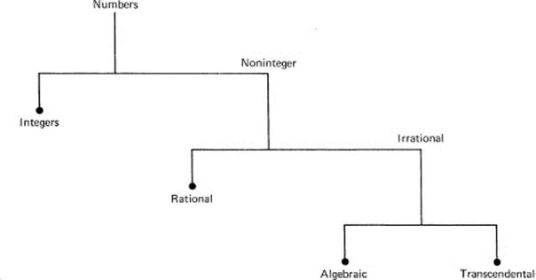
Figure 4.1-1 Types of numbers
The decision that a decimal representation corresponds to a number is in close agreement with what most people feel about what a number is. Never mind any elaborate definitions that may be made; such definitions come ultimately from the common feeling that numbers have decimal (or other number base) representations, and, conversely, decimal representations correspond to numbers. This approach leads to difficulties whose resolution we cannot go into here; that is, how we can be sure that these decimal representations obey the common rules of arithmetic? The average person believes they do, and we will leave it at that.
A polynomial is a linear combination of the powers of x with coefficients selected from some class. At the moment this class is the integers; later it may be the class of algebraic numbers or even the class of all real numbers. This is a special case of the general concept of a linear combination and is fundamental in mathematics. This concept is worth abstracting since it will occur many times in this book. First, we are given a collection of entities, call them Gi (these are the powers of x for a polynomial). Then a linear combination of the Gi can be written as
c0G0 + c1G1 + … + cnGn
where the ci, are selected from some other class of entities (they were the integers in the case from which we are abstracting).
The difference between algebraic and transcendental numbers can be described neatly in terms of polynomials with integer coefficients. Because an algebraic number is a solution of a polynomial of some degree n with integer coefficients, it follows that there is a linear combination (using integer coefficients) of the powers of an algebraic number such that the sum is identically zero. Therefore, all high powers of a particular algebraic number can be reduced, using its particular defining polynomial, to a sum of powers less than n. On the other hand, no finite linear combination of the powers of π using integer coefficients can be exactly zero. In mathematical symbols,
c0 + c1 π + c2 π2 + … + cn πn ≠ 0
for any integer n and integers ci (i = 0, 1, … , n), unless all ci are zero. See Section 4.7 for more details.
4.2 PHILOSOPHY
The idea that a continuous line is composed of points (which have no size) seems to be a contradiction. How can a line segment that has some length be composed of points that have no length?
As Zeno (336?–264? B.C.) dramatically put it in one of his famous paradoxes,
If at every instant the flying arrow is at some point, how is motion possible?
He created his paradoxes, apparently, not as denials of what we think we see in the real world, but rather to dramatize the logical difficulties that arise between the discrete and continuous views we have of the world.
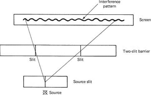
Figure 4.2-1 Two-slit experiment
A similar situation involving logical difficulties arises in the field of quantum mechanics in modem physics. In the famous two-slit experiment (Figure 4.2-1), the photon of light in passing through the two open slits seems to “know” how far the slits are apart because the resulting pattern on the photographic plate shows interference fringes whose detailed shape depends on the separation of the two slits. If one slit is closed, the photon goes directly through the other open slit and strikes the screen in the pattern of a small slit. Thus the photon exhibits “wave-like” properties, which produce the interference pattern. On the other hand, when the photon hits the photographic plate, apparently it hits as a particle, because when the photographic plate is processed we see that the corresponding molecule of silver is developed. Thus the photon exhibits “particlelike” properties. The explanation of this apparent paradox has not been clearly described in the more than 50 years since the start of modem quantum mechanics in 1925. The apparent contradiction between the two views is often resolved by what is called the complementarity principle, meaning that the two descriptions are to be regarded as complementary rather than competing descriptions.
So, too, we have the two descriptions: the continuous line has both length and is composed of points that do not have length. Mathematicians have found ways of defining things to evade the apparent paradox. This does not mean that the paradox has been solved, only that they have found ways of logically consistently evading the problem. Thus in mathematics you also face a complementarity principle: the continuous line is composed of discrete points.
As a result you are advised to meditate on the matter and to make up your own mind as to what you think about Zeno’s paradox of the flying arrows and the line being composed of points. As the student is usually told in a quantum mechanics course, “You will get used to it.”
By the identification (mapping) of the numbers with the points on a straight line, we establish an isomorphism (iso- means same; morphism means shape, form) between numbers and points. We want some features of one to be matched by similar features in the other; for example, each point on the line corresponds to a number and each number to a point on the line. The feature “greater than” corresponds to lying to the right.
4.3 THE IDEA OF A FUNCTION
In principle, the idea of a function is very simple. For each value of the independent variable (usually x) in some range of values (usually over the entire real line or some part of it, although, as we have already seen, sometimes only over a subset, say the integers), there is a corresponding value of the function (usually the value of y). In mathematical notation this is
y = f(x)
In other words, for a numerical function f(x) there are pairs of numbers (x, y) that give the correspondence between x and y. For each x in some admissible range, there is a single, unique value y.
This is a very large abstraction of your experience with particular functions. Consider the rich variety of functions you have already met in your life. If they are to be handled in any systematic fashion, together with all those you are going to meet in the future, some general concept and notation for a function are necessary.
Example 4.3-1
A number of familiar examples of functions are:
![]()
Their usual graphs are sketched in Figure 4.3-1.
If we pick a particular function, say
y(x) = x2 + 3
then you need to understand that the notation
![]()
means “in place of the original x you now use x + 1.” Again,
![]()
means in place of the original x you now use x3. Similarly,
![]()
The difficulty with the abstract idea of a general function is the same difficulty you met in beginning algebra. You were told that the symbol x was a general number. It took a long time for you to get used to the idea of a general number. We are in the same position now. You have had much experience with particular functions, even functions that were general in the sense of being a polynomial of degree n with both the degree and the coefficients of the function unspecified. But when we say no more than that y is a function of x, then we are dealing with a general function, and you need to make the same mental adjustment to this abstraction as you did for the general number. Many times we will finally get down to a specific function, but there will be times when we never specify much more than that y is a function of x. We have already deliberately used general polynomials on a number of occasions just to give you practice in handling generality. The generality gives vagueness, but it also gives power because the abstract functional dependence covers many special cases.
We will not be concerned with the most general possible functions; rather we deal with a limited class called piecewise continuous. This means that each function is composed of pieces, and each piece is continuous, where “continuous” at present means just what you think; when you draw a curve without lifting the pen or pencil, the curve is continuous (see Figure 4.3-2). “Piecewise” means that there may be discontinuities (jumps) between the pieces. We further restrict the definition to permit only a finite number of pieces for a finite range of x.
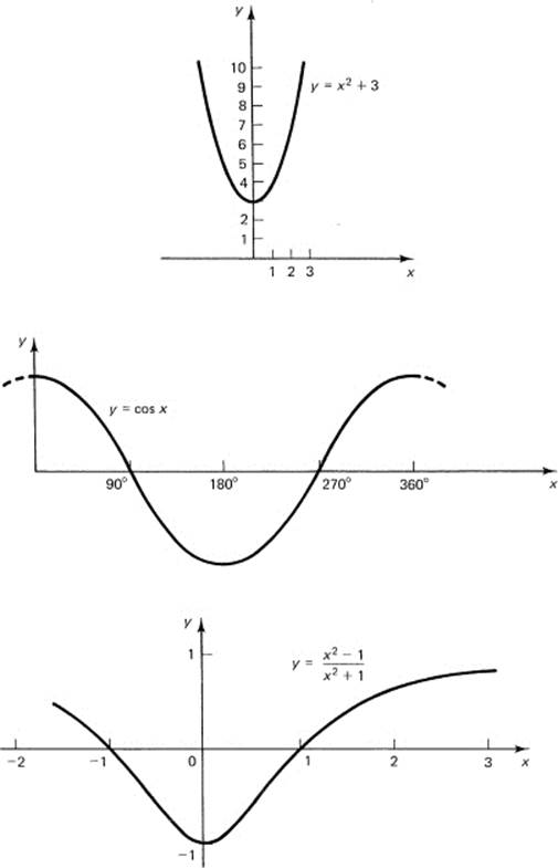
Figure 4.3-1 Some graphs of functions
Furthermore, we assume that each continuous piece is either nondecreasing or else is nonincreasing, usually called monotone increasing or monotone decreasing. See Figure 4.3-3 for an example. Occasionally, the words “strictly monotone increasing” are used to mean that there are no horizontal parts to the corresponding graph, and similarly for strictly monotone decreasing.
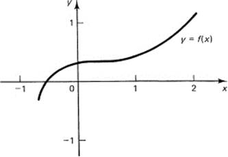
Figure 4.3-2 A Continuous function
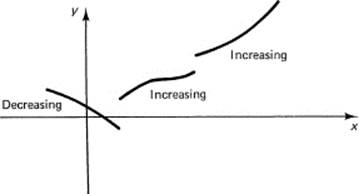
Figure 4.3-3 Piecewise monotone
Example 4.3-2
Consider the curve y = sin x for 0 < x < 360°. Figure 4.3-4 shows the graph. It can be broken into three parts. In the first one-fourth of the range, the values of the function form a monotone increasing function. In the middle half of the interval, the function sin x is monotone decreasing. Finally, in the last fourth the function is again monotone increasing.
Functions of a discrete variable together with functions that are piecewise monotone and continuous (Figure 4.3-5) can describe all the situations you are apt to meet when you apply mathematical models to real-world situations. More advanced mathematics is necessary to cope with the few situations that might arise when more complicated functions are studied. At this point, the mathematical technicalities to handle them do not seem worth the effort.
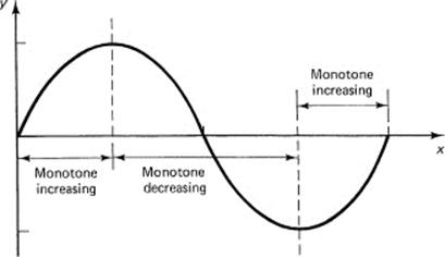
Figure 4.3-4 y = sin x
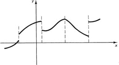
Figure 4.3-5 Piecewise monotone function
Example 4.3-3
The function
y(x) = {the greatest integer ≤ x}
is easily defined for all positive x and has a infinite number of horizontal pieces (see Figure 4.3-6). It is a monotone increasing function. For a finite range we allow only a finite number of places where there are discontinuities, where you can lift the pen or pencil and begin again. Evidently, we are excluding functions like
![]()
because near the origin the function has an arbitrarily large number of jumps. See Figure 4.3-7.
The reason for admitting discontinuous functions is that they occur frequently in practice. Examples are an on-off switch that controls a device, laws that become effective at a given date so that the corresponding social effects are being driven by a discontinuous cause, and many other situations in modem society where there is the sudden change of a cause or of an effect. If we are to model these with our mathematics, we need to allow gracefully for such functions.
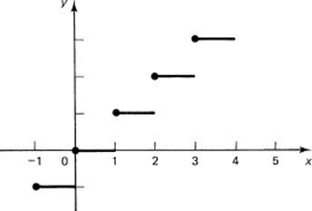
Figure 4.3-6 “Greatest integer in” function
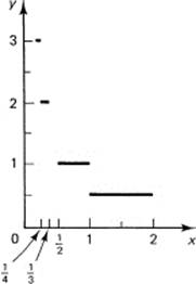
Figure 4.3-7 Greatest integer ≤ 1/x
Several troubles arise from the requirement that a function be single valued.
1.If you rotate the coordinate axes (Section 6.9*), then you may introduce multiple values for the same value x, and hence you no longer will have a function y = f(x).
2.At a point of discontinuity you are forced to omit at least one end value and hence later must compensate by supplying some technical details to obtain the missing value (Section 7.4).
3.As we will see in Chapter 22*, the sequence of approximating functions that approximate a discontinuous function comes closer and closer to supplying the vertical line bridging the discontinuity (see the figures in Section 22.3* for example).
4.We often need to deal with what would naturally be multiple-valued functions and are therefore forced to make artificial distinctions, which few mathematicians actually do in the “heat of doing mathematics.” It is only in the refined proofs that the care to restrict functions to single-valued functions is maintained.
On the other side of the argument, a number of troubles arise when you let functions have multiple values, and it is presently the custom to restrict the definition of a function to those that, for each x in some given range, have a single value.
In these days of computers, a function is often compared to a subroutine that takes one number in and delivers one number out. For example, some typical numerical functions are the square root, the sine, and the logarithm. In these words, the function of a function
![]()
means that the x is supplied to the square-root routine, and the square-root routine output is then supplied as input to the sine routine, whose output in turn is y.
EXERCISES 4.3
1.Extend “the greatest integer in” function to negative numbers.
2.Discuss the corresponding function, the smallest integer greater than or equal to x.
3.Discuss how the function cos x is composed of monotone pieces.
4.Is the function sin(1/x) an admissible function? Hint: Consider the neighborhood of the origin.
5.If f(x) = (1 – x)/(1 + x), find f(1/x).
6.If g(x) = (x2 + 2)/(x2 – 2), show that g(![]() ) = (x + 2)/(x – 2).
) = (x + 2)/(x – 2).
7.If f(t) = at, show that f(x)f(y) = f(x + y).
8.If y(x) = (1 – x)/(1 + x), show that y((1 – x)/(1 + x)) = x.
4.4 THE ABSOLUTE VALUE FUNCTION
Often, instead of wanting to know the position of a point on the line, we merely want to know how far it is from the origin. We measure this distance by the size of the number, the absolute value of the number, meaning
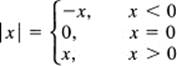
See Figure 4.4-1. Specific examples are
![]()
Figure 4.4-1 Absolute value function
Often we want to know the distance between two points a and b on a straight line. We have the simple formula for the distance function d( , ):
d(a, b) = |a – b| = |b – a|
This seems to be a reasonable measure of the distance along a line since:
1.It is nonnegative, d(a, b) ≥ 0.
2.It is zero if and only if the two points are the same point, d(a, a) = 0.
3.It is symmetric, meaning that the distance from one point to the other is the same as the distance from the second to the first point, d(a, b) = d(b, a).
The absolute value function provides an isomorphism (end of Section 4.2) between “the distance between numbers” and “the distance between points along the real line.”
Example 4.4-1
There are a number of simple relationships involving the absolute value function that will develop your skills in handling the idea. The first is the convenient relationship
![]()
since ![]() always means the positive square root. From the obvious relation
always means the positive square root. From the obvious relation
a ≤ |a|
we can deduce that
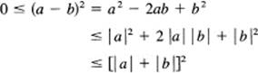
Therefore, we have the right-hand side of the following equation; by similar reasoning we get the left-hand side of
![]()
Since b could be any number, positive, or negative, or zero, we may change the sign of the b term if we wish. Thus we have, in general, after removing some minus signs,
![]()
Example 4.4-2
The particular function
![]()
For x > 0, it has the value y (x) = 1. For x < 0, it has the value y (x) = – 1. For x = 0, it is technically not defined because of the division by zero that would occur; but conventionally it is given the value y(0) = 0. See Figure 4.4-2. This is also called the signum function (the sign function) and is written
![]()
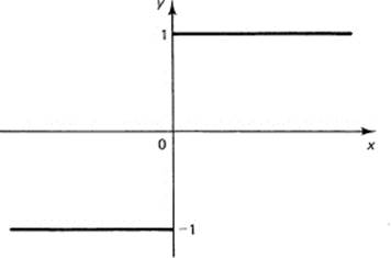
Figure 4.4-2 y = x/|x|
EXERCISES 4.4
1.Show that the function y(x) = |x|/x is the same function as that in Example 4.4-2.
2.Discuss the difference between y(|x|) and |y(x)|.
3.Discuss the Heaviside function y(x) = {x + |x|}/2.
4.Plot the function y(x) = {|x| – |x – 1| + 1}/2.
5.*Devise a function that is always 0 except that from 0 to 1 it rises along a straight line to the height 1, and then from 1 to 2 it goes back down to 0 along another straight line.
6.Is there a difference between x2 and |x|2?
4.5 ASSUMPTIONS ABOUT CONTINUITY
The concept of continuity arises from our intuition about drawing lines without lifting the pen (or pencil) and from our feelings about the continuous flow of time. We feel that at any place on the line, or at any moment in time, there should be a suitable number to mark it. We need to make this vague concept more definite.
We are not in a position to prove rigorously a number of properties about numbers and continuous functions, so we shall assume the following (in effect they define continuity):
1.If a formula (of the kind we will use) involving only continuous functions is true for all rational numbers, then it is also true for the irrational numbers. This is vague at present, but will become clear as we use it.
2.If in a closed interval a ≤ x ≤ b, also written as [a, b], a continuous function changes sign an odd number of times, that is, if
f(a)f(b) < 0
then there exists a number θ (Greek lowercase theta) such that
![]()
(meaning there exists at least one number θ where the function is zero).
3.In a closed interval [a, b] a continuous function takes on its maximum; that is, there exists at least one number θ (although it is not the same θ as above) for which f(x) is at least as large as for any other number in the interval. In mathematical notation, there exists a θ such that
![]()
These are the three properties we assume about continuous functions and the existence of numbers; they assure us that when we use continuous functions in these ways there is always a number waiting for us. We will therefore not be in the position of Pythagoras who found that among the everywhere dense rationals there was no ![]() . This does not mean that there could not be other processes for which there would be no corresponding numbers, merely that if we use only the above processes we will always find a suitable number waiting for us.
. This does not mean that there could not be other processes for which there would be no corresponding numbers, merely that if we use only the above processes we will always find a suitable number waiting for us.
We need one further assumption:
4.For any convergent sequence of numbers, the limit is a number, where by the words “convergent sequence” at the moment we mean something similar to taking more and more decimal digits of a number and having it “converge” to the number, or similar to a geometric progression when the rate r is less than 1 in size and the number of terms is indefinitely increased. See Examples 3.6-2 and 3.6-7, as well as Section 7.2 and Chapter 20.
We need to examine these assumptions to see how well they agree with our intuitive feelings. If they do not agree then we must either change the assumptions or else our feelings as to what continuity is. The first assumption says that since the rational numbers are everywhere dense any further numbers that we put on the line should not have wildly different properties when we use continuous functions. In this way we assert that we can operate with the new numbers without proving that the rules for rationals also apply to the irrationals. A rigorous treatment of the subject would require proofs of these properties, but we are not in a position to prove them in a first course in calculus. We need this principle to extend the laws of exponents (Section 3.8) from the rational exponents to irrational exponents, for example, that there exists a number (given an x > 0)
![]()
We also need it so we can say that the rule
xaxb = xa + b
is true for all real numbers a and b.
The second assumption merely says that a continuous curve cannot pass from positive to negative values without taking on the value 0 for some number x. This is a reasonable description of our idea of continuity. We are assured by this assumption that there is always a number where a continuous function that changes sign takes on the value 0, that there will be a number waiting for us; we will not be in the position of Pythagoras when he first met ![]() . We used this assumption in Section 3.5 when we found certain irrational numbers.
. We used this assumption in Section 3.5 when we found certain irrational numbers.
The third assumption also seems reasonable, that in a closed interval a continuous function takes on an extreme value somewhere in the interval, perhaps at the ends. The assumption assures us that there is a number where the function takes on its extreme value, something that we will often need later.
The last assumption about the existence of a limit that is a number requires a clearer idea of convergence (see Chapter 20) before we can say that we believe it. It does seem, however, to be a plausible assumption.
4.6 POLYNOMIALS AND INTEGERS
The familiar polynomials are the simplest continuous functions, and they play a role very much like the integers. In both cases they are the elementary pieces from which more complex expressions are built. Both the integers and polynomials are closed under the operations of addition, subtraction, and multiplication; the results of these operations lie within their own class. There is a strong similarity between polynomials and the integers. In this book, most of the time, we are concerned with real numbers and real polynomials. The exceptions are specifically mentioned when they occur.
It is the operation of the division of two integers that requires the extension to the rational numbers (to fractions), and, similarly for polynomials, division leads to the class of rational functions,
![]()
where N(x) and D(x) are polynomials. Both the integers and polynomials have the ideas of factorization, primeness, and reduction to lowest form. For example, in the class of polynomials with real coefficients, x2 + 1 is a prime polynomial (has no real factors other than 1 and itself).
Rational functions dominate many parts of mathematics and statistics. The reasons that make the rational numbers prominent in arithmetic are similar to those that cause the rational functions to play a prominent role in much of mathematics. There are, similar to the case of numbers, functions that are not rational functions. For example, the trigonometric functions are transcendental functions, meaning that they are not the solution of any algebraic equation
![]()
where f(x, y) is a polynomial in the two variables x and y. See end of Section 4.7.
Abstraction 4.6-1.
Euclid’s algorithm. When we see the preceding similarities, it is natural to ask, “How far can we carry the similarities between the integers and the polynomials?” We have already compared a great many properties. What else could we compare? Euclid’s algorithm comes to mind as a method of finding the GCD (greatest common divisor) of two integers. Does it apply to polynomials? We have only to reexamine the proof in Section 3.2 and identify the ri, and the qi in the section with the corresponding polynomials. Thus, as we reread the proof, each time we see an rior a qi we have to think the polynomials ri(x) and qi(x).
Following along the proof, we see that dividing one polynomial by another leaves a remainder of degree less than that of the divisor. Evidently, the integer being forced to zero in the original proof corresponds to the degree of the polynomial being forced to zero (a constant) in the new proof. An examination of the proof shows that all the divisibility arguments are the same in both cases.
We conclude that, with a simple change in understanding, Euclid’s algorithm applies to polynomials just as it did for the integers. Evidently, Euclid’s algorithm is not concerned with just integers; it applies to any entities that have certain properties. We will not, at this point, give the least properties that suffice for the algorithm to work, but the above shows that methods developed for some things (integers) can often apply, sometimes with slight changes, to other things (polynomials).
EXERCISES 4.6
1.Define a polynomial.
2.If P(x) = x3 + x + 1 and Q(x) = x2 – 1, find P(x) + Q(x), P(x) – Q(x), and P(x)Q(x).
3.Find the GCD of x3 + 2x2 + 2x + 1 and x2 – 1. Ans.: x + 1.
4.Find the GCD of x4 + 1 and x2 – ![]() x + 1. Thus you can factor x4 + 1 in terms of real polynomials.
x + 1. Thus you can factor x4 + 1 in terms of real polynomials.
5.*Generalize Exercise 4. Ans.: You can always factor xk + 1 for k > 2 in terms of real polynomials. Hint: The odd powers always have a factor of x + 1, and in the even exponent cases, writing x to some suitable even power as t, you can get either an odd power for the t or else an exponent of 4.
6.*Fill in all the details of Euclid’s algorithm for polynomials.
4.7 LINEAR INDEPENDENCE
In Section 2.5 we proved that a polynomial in x (a linear combination of a finite number of the powers of x) cannot be identically zero for all integer values of x unless all its coefficients are zero. This is a very useful result and is worth looking at more closely to see how much the requirements can be weakened. When a linear combination of functions (Section 4.1) is identically zero (for all values of the variable), we say that the functions are linearly dependent. In the abstract notation of Section 4.1, if the ci (not all zero) and the Gi(x) are given, then if
![]()
for all x in some set (possibly an interval), then the Gi(x) are linearly dependent; there is a linear relationship between the Gi(x). If there is no set of coefficients ci not all zero, such that the linear combination is identically zero, then the functions are said to be linearly independent (over that set of points).
In the case of polynomials, the Gi are the powers of x, and ci are the constant coefficients
![]()
Linear independence is a powerful tool. For example (as we will soon prove), from the statement that a polynomial of degree n is zero for at least n + 1 values, you can set each coefficient equal to zero separately and get n + 1 separate equations.
We turn to the proof of this important statement. Most students remember something about a polynomial of degree n having exactly n zeros. This suggests that if the polynomial were zero (vanished) at n + 1 points it would have to be identically zero; every coefficient would have to be zero. This kind of proof would be based on the fundamental theorem of algebra that a polynomial of degree n has exactly n zeros, real or complex. This theorem is difficult to prove, so we will base our examination of the situation on a simpler result, the factor theorem.
The factor theorem states that if for a value x = a the polynomial Pn(x) is zero, that is, if
![]()
then the polynomial is divisible by the factor x – a.
The proof is based on the observation that (see Section 2.6 under geometric progressions)
![]()
This can be seen directly by multiplying out the right-hand side and noting that all the terms, except the first and last, cancel. This is a typical ellipsis proof. If a is a zero of Pn(x), meaning that Pn(a) = 0, then we can write
![]()
since the second term on the right is zero by assumption. If we now write out the general polynomial P(x) in some detail, we have
![]()
then
![]()
and each term is divisible by x – a. Hence
![]()
where Pn-1(x) is some polynomial of degree n – 1. Thus, if a polynomial vanishes for some value x = a, then it has the factor x – a.
A variant of this result is called the remainder theorem, which states that, if you divide a polynomial P (x) by the factor x – a, then the remainder is P (a). This is easily seen from the division when written in the form
![]()
where Q(x) is the quotient and r is the remainder (which is a constant). If you set x = a in this equation, you get the result
![]()
From the factor theorem we see that, corresponding to each distinct number xk for which the polynomial vanishes, P(xk) = 0, there is a factor
x – xk
of the polynomial Pn(x). Since each (distinct) number xk cannot make any one of the already found factors zero, and since the product of them with the remaining polynomial must vanish at any other zero, it follows that the new polynomial has all the other zeros that have not already been used up to this point. We can therefore apply the factor theorem to the result. Now a polynomial of degree n cannot possibly have more than n factors of degree 1. Therefore, if there were n distinct values ak for which the original polynomial Pn(x) vanished, it would have the form
![]()
If there are n + 1 distinct zeros, then cn = 0 and the polynomial is identically zero. We have now proved that:
If a polynomial of degree n has n + 1 distinct zeros, then it is identically zero.
Since a polynomial is a linear combination of the powers of x, another way of stating the above result is that the n + 1 powers of x staring from x0 = 1 and going up to (and including) xn are linearly independent over any set of n+ 1 points. No linear combination of them with numerical coefficients can be zero at n + 1 points unless all the coefficients are zero. We have reduced the condition of Section 2.5 that the polynomial be zero for all sufficiently large integers to the much simpler condition that the polynomial vanish at n + 1 points. This has many important consequences.
Example 4.7-1
Unique representation. One example of the use of this result tells us that any n + 1 distinct samples of a polynomial of degree n suffice to determine the polynomial; we are assured that we will always be able to solve for the coefficients when we use undetermined coefficients.
To prove this statement, two things must be shown: first, that there is at least one polynomial through the given data, and, second, that there is not more than one such polynomial. To prove the first part, we use mathematical induction. As a basis for the induction, we observe that given n + 1 samples
![]()
then for n = 0 we have
![]()
as the required polynomial. When n = 1 there are only two points, and the first-degree equation
![]()
is the solution. This can be seen by substituting x0 and x1 and evaluating the right-hand side. We see the beginning of a recursive proof.
In the mathematical induction pattern, we now assume that there is a polynomial of degree n – 1 through any n points, and then start with the n + 1 points and a polynomial of degree n. Let this polynomial be
![]()
We then write this as
![]()
where Qn–1(x) is to be determined. We see that this expression is satisfied at the value xn. For all n other values, we compute the value of
![]()
By the induction hypothesis, this polynomial Qn–1(x) can be found and the induction is proved (since we have the basis for the induction for both n = 0 and n = 1).
For the second part of the proof, if there were two or more such polynomials, say P(x) and R(x), that satisfied the given data of n + 1 points, then the difference P(x) – R (x) would be zero at the n + 1 points; hence it would be identically zero. Thus the result is proved.
Thus any n + 1 samples of a polynomial of degree n are equivalent to the polynomial. This means that we may use the samples of the polynomials as if they were the polynomial with no loss of information. The result says, in different words, that if two polynomials are equal to each other for enough values, one more than the highest degree term occurring, then they are equal for all values. We can use the samples of the function to determine the polynomial.
Example 4.7-2
Given the samples (–1, 0), (0, 2), (1, 2), and (2, 4), construct the polynomial having these values (Figure 4.7-1). We could proceed as in the above proof, which involves a lot of special memory on your part, or else we could use the method of undetermined coefficients, which is a very general method. Given four samples, we need a polynomial with four undetermined coefficients, that is,
![]()
We next impose the four conditions that the data satisfy the equations.
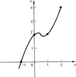
Figure 4.7-1 ![]()
|
Point |
Condition |
|
(−1, 0): |
a(−1)3 + b(−1)2 + c(−1) + d = 0 |
|
(0, 2): |
a(0)3 + b(0)2 + c(0) + d = 2 |
|
(1, 2): |
a(1)3 + b(1)2 + c(1) + d = 2 |
|
(2, 4): |
a(2)3 + b(2)2 + c(2) + d = 4 |
From the second equation, it is immediately clear that d = 2. Using this, rewriting the other three equations, and dividing out the factor 2 in the bottom equation, we get
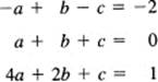
Add the top two of these three equations to get immediately b = –1. Take the top and third equation with this value of b substituted in, and we have
![]()
Subtract the top from the second of these, and we have
![]()
This gives, from the upper of the two equations,
![]()
and the coefficients are now known:
![]()
We can check this easily by substituting the sample values to see if we get the right values; we get
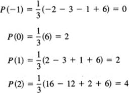
Thus we have found the polynomial and verified the fact that it satisfies the given sample values.
Linear independence is a negative property; it asserts the nonexistence of a set of coefficients. When a set of nonzero coefficients exists such that the sum of some set of functions is zero for the corresponding interval (or set of points), then the functions are linearly dependent (over some interval or set of discrete points). Linear dependence asserts that there is a linear relationship between the functions, and therefore they are not suitable for the representation of the general function of some class because there are one or more hidden linear relationships among the representing functions. Linearly independent functions, on the other hand, are often a suitable basis for representing things. Linear independence is an idea that we will often use and is a central concept in mathematics.
We can now prove that the function y = sin x cannot be the solution of an algebraic equation (a polynomial in two variables x and y)
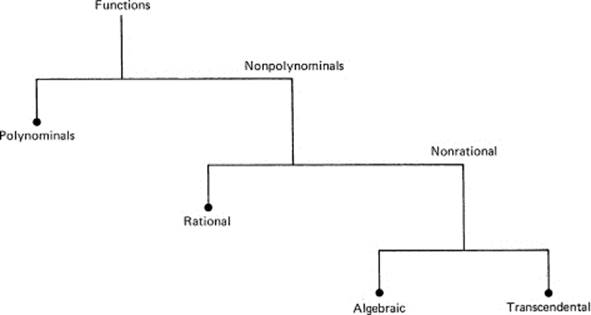
Figure 4.7-2 Types of functions
![]()
since for a fixed y less than 1 in size there are infinitely many solutions x of y = sin x (xk = x0 + 360°k for all integers k and x0 is any particular solution), while a polynomial can have (for a fixed y) only a finite number of solutions (zeros). Thus the trigonometric function
![]()
must be a transcendental function (it cannot satisfy an algebraic equation in two variables). A similar proof applies to any other periodic function (except a constant). Figure 4.7-2 is to be compared with Figure 4.1-1.
EXERCISES 4.7
1.Define linear independence.
2.Given that x = 2 and x = 3 are zeros of P(x)= x3 – 9x2 + 26x – 24, find the factors of P(x).
3.Given that x = 1 and x = –1 are factors of P (x) = x4 – 5x3 + 5x2 + 5x – 6, find the factored form of P(x).
4.Find the polynomial through the data (–1, 2), (0, 1), (1, 5).
5.Find the polynomial through (–2, –8), (–1, –1), (0, 0), (1, 1), and (2, 8).
6.Show that y = cos x is a transcendental function.
7.Show that in general any periodic function (other than y = c) is a transcendental function.
4.8 COMPLEX NUMBERS
Mathematicians, scientists, and engineers are all agreed that it is very unfortunate that ![]() = i is called an imaginary number, and that numbers like 2 + 3i are called complex numbers. Had they been called numbers of the second kind, then probably there would be much less resistance on the part of the beginner to accepting them as numbers. Experience has shown that these numbers are as “real” as any other numbers. In particular, in many fields of knowledge, complex numbers explain and unite many different things that at first seem to be unrelated.
= i is called an imaginary number, and that numbers like 2 + 3i are called complex numbers. Had they been called numbers of the second kind, then probably there would be much less resistance on the part of the beginner to accepting them as numbers. Experience has shown that these numbers are as “real” as any other numbers. In particular, in many fields of knowledge, complex numbers explain and unite many different things that at first seem to be unrelated.
Complex numbers first arose in connection with the solution of the quadratic equation
![]()
using the formula for the roots (derived in Example 6.3-2 if you have forgotten it)
![]()
If the discriminant b2 – 4ac > 0, then the quadratic equation has two real and distinct roots: If b2 – 4ac = 0, then both roots are equal to –b/2a. If b2 – 4ac < 0, then the formula for the roots can be written as
![]()
where i = ![]() The roots are then complex numbers, each root being the complex conjugate of the other (“conjugate” means that the sign of the imaginary part is changed).
The roots are then complex numbers, each root being the complex conjugate of the other (“conjugate” means that the sign of the imaginary part is changed).
As a general rule, you handle complex numbers just as you would handle rational numbers, when you also had a ![]() . In such a system, we let a and b be rational numbers and adjoin the. irrational number
. In such a system, we let a and b be rational numbers and adjoin the. irrational number ![]() . Suppose
. Suppose
![]()
are two such numbers with rational coefficients a, b, c, and d. The two terms of each number cannot be combined because, as we proved in Section 3.4, a fraction cannot be equal to ![]() . If we add the two numbers, we get
. If we add the two numbers, we get
![]()
as the sum, and similarly for the difference. When we multiply the two numbers, we get
![]()
We merely replace (![]() )2 = 2 whenever it arises. In a similar fashion, all numbers involving higher powers of
)2 = 2 whenever it arises. In a similar fashion, all numbers involving higher powers of ![]() can be reduced to a rational number plus a rational number multiplied by
can be reduced to a rational number plus a rational number multiplied by ![]() .
.
For division the matter is slightly more complicated. Given the quotient
![]()
we multiply both numerator and denominator by c – d![]() . We get
. We get
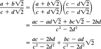
Thus we have reduced the quotient to the form of a rational number plus a rational number multiplied by ![]() .
.
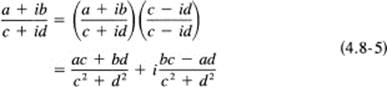
Complex numbers are handled exactly the same way except that i2 = –1. We do not want exceptions in our methods when we can avoid them. Given
![]()
their sum is
![]()
Their product is
![]()
For the quotient we use the conjugate of the denominator (c – id) as the multiplicative factor for both the numerator and denominator:
One rule that complex numbers do not obey is the old rule for real numbers:
![]()
For complex numbers we would have, if they did,
![]()
which is obviously false.
We see that these new numbers satisfy most, but not all, of the expected rules of algebra. For example, the quadratic equation (4.8-1)
![]()
can be factored into the two factors
![]()
When multiplied out, this gives
![]()
and a comparison with the original equation (4.8-1) shows that the sum of the roots is –b/a, while the product of the roots from (4.8-2) is c/a. In the complex form we easily see that the sum of the two conjugate roots is indeed –b/a. It remains to check the product of the two roots (4.8-2):
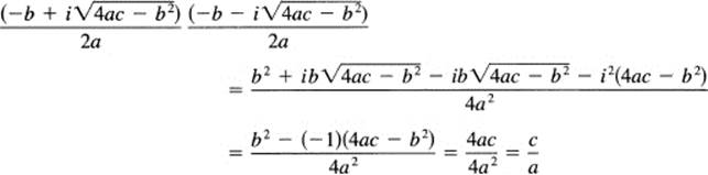
as it should. Thus the formal replacement of i2 = –1 is all that is new.
Using the concept of linear independence, we can say that the real and imaginary oarts of a complex number are linearlv independent since if
![]()
it follows that (since a real number a cannot be equal to an imaginary number b) both a = 0 and b = 0. Similarly, if two complex numbers are equal
![]()
Then
![]()
As we noticed before, when we extend a class of numbers to a larger class we often lose one or more properties. For example, in going to complex numbers, we lost (4.8-6)
![]()
In going from the real numbers to the complex numbers, we also lose the order relationship. Real numbers have the property that, given any two numbers a and b, we have one of the three possibilities
![]()
We further have (Section 3.3) that, if c > 0 and a > b, then
![]()
The order relationship is maintained if we multiply by a positive number.
For complex numbers there is no such ordering. To prove this, we argue as follows. Suppose there were an order relation among the complex numbers; then consider the quantity i. It is surely not equal to zero. If we first assume that
![]()
then multiplying by i > 0 we would have
![]()
which is false. If we next assume that
![]()
then multiplying by i would reverse the inequality, and we would again have
![]()
Thus the complex numbers cannot be ordered.
In place of ordering, we still have the concept of size, called the absolute value or the modulus (modulus refers to distance, Roman origin) of the number. Given a + ib, we define the absolute value as
![]()
Thus the number and its conjugate have the same “size” (modulus). We often use the convenient form
![]()
In words, the square of the modulus of a complex number is the product of the number and its conjugate.
We see that the complex numbers are really not so strange as they first seem. You handle them much as you handle a quadratic irrationality like the ![]() when dealing with rational numbers. The only two things to watch for are that the square root of a product is not necessarily the product of the square roots, and that the numbers cannot be strictly ordered; but the modulus, or absolute value, plays a very similar role in their arithmetic and algebra.
when dealing with rational numbers. The only two things to watch for are that the square root of a product is not necessarily the product of the square roots, and that the numbers cannot be strictly ordered; but the modulus, or absolute value, plays a very similar role in their arithmetic and algebra.
EXERCISES 4.8
Evaluate the following:
1.(3 + 4i) + (4 – 3i).
2.(3 + 4i)(4 – 3i).
3.(3 + 4i)(3 – 4i).
4.(2 + 3i)/(4 – 3i).
5.(6 + 3i)/(2 + i).
6.(a + ib)2.
7.(a + ib)3.
8.(a + ib)4 (a – ib)4.
9.Show that (a + ib)2(a – ib)2 = |a + ib|4.
10.If a + b ![]() = c + d
= c + d![]() for rational a, b, c, d, then show that a = c and b = d.
for rational a, b, c, d, then show that a = c and b = d.
11.Show that (1/2 + i![]() /2)3 = –1.
/2)3 = –1.
12.Show that (![]() /2 + i/2)3 = i.
/2 + i/2)3 = i.
13.*Find the square root of a + ib. Hint: Set it equal to c + id, square both sides, equate coefficients, eliminate one letter, solve the resulting quadratic in the square of the variable, and take the positive root so that the variable itself will be real.
14.*Show how to reduce any high power of a complex number to the form u + iv.
15.*Show that any polynomial in a + ib qan be written as u + iv where u and v are real.
16.*Show that Q(x) = [x – (a + ib)][x – (a – ib)] is a real quadratic.
17.*Generalized remainder theorem. Show that for complex numbers x, P(x) = Q(x)q(x) + r1x + r0, where Q(x) is a real quadratic, q(x) is the quotient, and r1x + r0 is the remainder.
18.*Show that to evaluate a polynomial for a complex number P (a + ib) you can (1) form the real quadratic as in Exercise 16, (2) divide the polynomial by the quadratic as in Exercise 17, and then (3) the remainder at x = a + ibis the value of the polynomial.
4.9 MORE PHILOSOPHY
Mathematics often gives the appearance of certainty. Furthermore, people wish to believe that somewhere there is certainty in this world of constant change—from moment to moment even science changes its rules and pronouncements—and mathematics seems to offer a haven from constant change. But this certainty is an illusion! See references [D], [K–2], and [L].
Consider the sentence (compare with Section 1.6)
This statement is false.
What are we to make of it? It seems to contradict itself! If it is true, then it asserts that it is false, and if the sentence is false, then it is a true statement. Even a simple grammatical sentence can contradict itself. How about mathematics? In mathematics we have occasionally managed to show that, if one set of assumptions is not self-contradictory, then another set is not, but we have not (as yet) shown that simple arithmetic is consistent, that from the same problem, and using only legitimate arithmetic, we cannot get two different answers. We also know that if a set of assumptions contains an inconsistency then any result can be obtained!
We do know that:
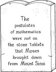
The postulates of mathematics were made by humans and are subject to human frailty.
Mathematicians also know that at the logical foundations of mathematics there are many paradoxes, meaning that we can get, by reasoning in accepted ways, results that we do not like. Although mathematics is heavily concerned with symbols, we know that we cannot even define the concept of a symbol; we can only give examples of what we mean. Furthermore, from the Godel theorems we believe that there are strings of symbols whose truth or falsity we cannot determine within any reasonably rich system of symbols (“cannot determine” in the same sense that ![]() cannot be a rational number).
cannot be a rational number).
Add to all this the simple fact that we use mathematics to “model” the real world of our senses. We begin with experience, model it in mathematical symbols, apply more or less standard methods of mathematics, and then try to reinterpret the results back to the real world of experience. The gaps between the external world of our senses and the internal world of our symbols are very large indeed, and we have (as yet) no idea of how to make a secure connection in either direction. See Figure 4.9-1.
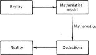
Figure 4.9-1 Use of mathematics
But when all this is said and accepted, we also know from experience (as given briefly in Section 1.3) the effectiveness of mathematics. We do risk human lives and large sums of money on the results we obtain from mathematics. It is useless to say that since we cannot be sure then we should take no action. To take no action is as definite an action as any other action! Passive resistance in the hands of Gandhi was a very aggressive weapon indeed. The refusal to take actions in the presence of uncertainty can be very dangerous and harmful to you and/or others.
What can the reasonable person do? You can neither sensibly believe everything that comes from mathematics nor believe nothing. You are left to think about the assumptions in the form of postulates and about the logic you use along the way, and then decide when it is prudent to believe and when it is prudent not to believe. Mathematics, much as you may wish that it would, does not give certainty; it is by no means what it appears on the surface. There is a strong tendency for most people to gloss over these awkward aspects of mathematics and to go forward without questioning. But for those who expect to use mathematics to shape actions in the world, serious attention to these difficulties is necessary.
We have tried to clearly label assumptions and the forms of logic we have used, and we will from time to time highlight results that are often ignored. It seems necessary to actively combat both the illusion of, as well as the desire for, infallible mathematics.
4.10 SUMMARY
In this chapter we have carefully introduced the geometric representation of numbers (although we have used it implicitly before). We have not slighted the difference between our ideas of a uniform continuous line and the discrete nature of the number system and have left the matter for your consideration. If you are to develop new applications of mathematics, it may well depend on your understanding how numbers do or do not represent the things of interest in your chosen field. You may have to convince both yourself and others that the classical model of mathematics is, or is not, relevant.
The next concept, the idea of a function, is not easy to master, but it is essential that we be able to deal with broad classes of functions and not get caught endlessly with learning about each specific function. The failure to grasp this central idea will greatly hinder you later. We applied the concept of a function to a number of special cases to illustrate it, in particular, the useful absolute value function y = |x|.
We then took up the concept of continuity, which is simply an abstraction of your experiences with time and a continuous line. We could not use much rigor and were reduced to “hand waving” and saying, “You see that….” But if the rigorous approach did not agree with our intuition, then it would (probably) be altered.
We also took up the topic of complex numbers, which needlessly frightens the beginner (mainly because of the names “imaginary” and “complex”). We used the analogy with rational numbers and ![]() . Indeed, if you know how to handle these, then complex numbers are exactly the same except that you use i2 = – 1. Complex numbers are important for many reasons. One reason is that the two parts, the real and the imaginary, are linearly independent so that a single complex equation is equivalent to two real equations, a great gain in many situations. But more important, as you will see in Section 21.5 and Chapters 22* and 24, complex numbers provide a unity for what on the surface seems to be diversity.
. Indeed, if you know how to handle these, then complex numbers are exactly the same except that you use i2 = – 1. Complex numbers are important for many reasons. One reason is that the two parts, the real and the imaginary, are linearly independent so that a single complex equation is equivalent to two real equations, a great gain in many situations. But more important, as you will see in Section 21.5 and Chapters 22* and 24, complex numbers provide a unity for what on the surface seems to be diversity.
Finally, we again remind the reader that mathematics is not the certain thing that many people believe, or at least wish were true. It is essential that you learn to both believe and disbelieve at the same time; I have long observed that great scientists can tolerate ambiguity, and you need practice in this important trait.