Methods of Mathematics Applied to Calculus, Probability, and Statistics (1985)

Part I. ALGEBRA AND ANALYTIC GEOMETRY

Chapter 5. Analytic Geometry

5.1 CARTESIAN COORDINATES

We have just seen in Chapter 4 that there is an isomorphism (iso-, same; morphism, form) between the real number system and the geometry of a straight line (a one-to-one correspondence between parts of each with some properties also corresponding). For example, the absolute value function measures both the distance between points and the distance between numbers.

We now turn to a review of the geometry of the plane. It is natural to use a pair of mutually perpendicular lines as the basis for locating points. These lines are called the coordinate (co-ordinate) axes and are typically labeled xfor the horizontal and y for the vertical line. As shown in Figure 5.1-1 the values on the coordinate axes of a point in the plane are the numbers where the perpendicular projections of the point fall on the axes. Thus, to each point in the plane there is a unique pair of numbers, and to each pair of numbers there is a unique point. In the jargon of mathematics, there is a one-to-one correspondence (isomorphism) between the points of the plane and pairs of numbers. The number pairs are conventionally written

(x, y)

The names abscissa and ordinate are given to the x and y coordinates. (Note that in the parentheses and in the dictionary x precedes y and abscissa precedes ordinate.)

Coordinate systems with nonperpendicular axes are occasionally convenient, but the advantages of the standard perpendicular ones are so great that they are almost always used. Once in awhile curves rather than straight lines are used as the coordinate axes. Unless otherwise stated, the coordinate systems used in this book will always be the mutually perpendicular straight lines.

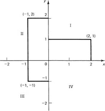
Figure 5.1-1 Coordinate system

In geometry we think of the plane as being isotropic (iso-, same; tropic, turning, changing), the same in all directions and all positions. Thus a translation of the coordinate system or a rotation of the axes does not change the geometric properties of things, but clearly does change the numerical values of the coordinates of a particular point. Felix Klein (1849–1925) in 1892 suggested that the various geometries be classified according to the set of transformations that left the corresponding geometrical elements unchanged. For Euclidean geometry, these transformations are (1) translations, (2) rotations, and (3) a reflection in a line. The geometrical elements are points, lines, triangles, circles, areas, and so on. Orientation is not an element of classical Euclidean geometry, since reflections are permitted and they reverse the orientation in the plane (recall Section 1.2).

As your algebra teacher probably said, “You cannot add apples to oranges,” and hence the ability to rotate the coordinate system implies that the same size and kind of units are used on both axes. If both axes are lengths, then rotation is a possible transformation, but if one axis is measured in dollars and the other is measured in units of time, then a rotation makes no sense. As noted earlier (end of Section 4.3), the definition of a function says that there must be a single value for y for each value of x that is permitted, and this can cause trouble when you rotate the axes of the coordinate system.

The coordinate axes divide the plane into four quadrants. Conventionally, they are numbered, I, II, III, and IV in a counterclockwise direction, as shown in the Figure 5.1-1. Thus, in the quadrant II, x < 0 and y > 0, while in quadrant IV, x > 0 and y < 0. In quadrant III, both coordinates are negative.

EXERCISES 5.1

1.Plot the points (a) (3, –4); (b) (4, –3); (c) (0, 0); (d) (0, –3).

2.Describe the coordinates of points on the x-axis. On the y-axis.

3.Describe the coordinates of points on the 45° line. On the 135° line.

4.Connect the four points (1, 0), (0, 1), (–1, 0), and (0, –1) in order. What is the shape?

5.Connect the four points (1, 1), (1, −1), (− 1, − 1), and (− 1, 1) in the natural order. What is the shape?

5.2 THE PYTHAGOREAN DISTANCE

In geometry it is not the values of particular coordinates that matter, but only the relationship between coordinates of different points. Therefore, we need a measure of the distance between two points p₁ and p₂. The coordinate axes are perpendicular, so we use the Pythagorean (Euclidean) distance, the length of the diagonal of a rectangle, as the measure of this distance. See Figure 5.2-1. We will later see that this is the only distance measure that makes sense in geometry when both rotation and translation are allowed. If the two particular points are p₁ = (x₁, y₁) and p₂ = (x₂, y₂), then the square of the distance between them is given by

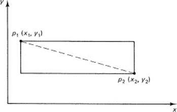
Figure 5.2-1 Pythagorean distance

Example 5.2-1

If the two points are (3, 4) and (5, –2), then the distance

This distance function (5.2-1) effectively commits you to using the same units on each of the coordinate axes; you cannot speak intelligently about the distance between different points on a dollar versus year curve.

This Pythagorean distance function has the properties you would expect a distance function to have:

1.d(p₁, p₂) ≥ 0

2.d(p₁, p₂) = 0 if only if p₁ = p₂

3.d(p₁, p₂) = d(p₂, p₁)

4.d(p₁, p₂) + d(p₂, p₃) ≥ d(p₁, p₃)

In words, the first says that the distance between points is never negative; the second says that the distance is zero if and only if the two points are the same point; the third says that the distance from one point to a second point is the same as in the opposite direction; while the fourth says that the distance obeys the triangle inequality, that is, the sum of any two sides is greater than, or equal to, the third side of a triangle since a straight line is the shortest distance between two points. Recall that in Section 4.4 the absolute value function had all of these properties (property 4 trivially).

If we look at the definition (5.2-1) of the distance between two points, from the algebraic point of view we see immediately that, since the square root is always taken to be positive, the first three conditions are satisfied. The fourth is harder to prove algebraically.

EXERCISES 5.2

1.Find the distance from the origin to each of the four points in Exercise 5.1-1.

2.Find the distance from (1, –1) to (–1, 1). Ans.: d = 2

3.Find the distance between each pair of points: (2, 2); (0, 1); (1, 0).

4.Check the triangle inequality for the points (0, 0), (3, 4), and (6, 8). What does this mean geometrically?

5.Show that the three points (1, 0), (0, 3), and (2, 2) form an isosceles triangle (at least two sides equal in length).

6.*Consider the function D(x, y) = | x₂ – x₁ | + | y₂ – y₁ |. Is this a suitable distance function? Why?

5.3 CURVES

Given a function

y = f(x)

then, for each real number x (of those that are suitable), there is a corresponding y, and the x and y may be regarded as the coordinates of a point. Thus corresponding to a function there is a set of points in the plane. We call the set of points the locus (loci is the plural of locus). There is, therefore, a correspondence between equations and single-valued curves in the plane; each locus is a curve consisting of all pairs of numbers (points) that satisfy its equation

y = f(x)

By convention, straight lines are regarded as being curves. Note that there are equations that are not single valued.

Example 5.3-1

The equation x² + y² = 1 is the locus of all points one unit from the origin (Figure 5.3-1).

This is Descartes’ (1596−1650) great observation and is the basis of analytical geometry. He noted that algebra and geometry correspond, that there is (almost) a complete isomorphism between them. For example, in Figure 5.3-2 there are two curves and they have a point in common. It follows that the corresponding equations have a solution in common. And conversely. This simple, elegant, and fundamental observation by Descartes is why the perpendicular coordinate system is called Cartesian coordinates.

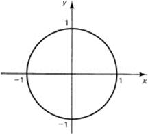
Figure 5.3-1 x² + y² = 1

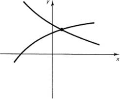
Figure 5.3-2 Intersection of two curves

Example 5.3-2

As a concrete example, consider the two linear equations (linear means that all the terms in the equation are of first degree or lower)

Figure 5.3-3 shows the corresponding curves (loci) of these equations; in this case they are straight lines, as we will soon prove. (This is probably the source of the word “linear” that is used so much in mathematics.) In the algebraic approach, we subtract the second equation from the first to eliminate the y term. We get

Put this solution (coordinate) x = 1 in either equation and you find that y = –1. Thus the algebraic solution of the two equations (1, −1) also gives the coordinates of the common point of the two lines (1, –1).

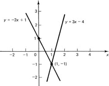
Figure 5.3-3 Intersection of two straight lines

To repeat the idea, Descartes showed that we can take problems in algebra and convert them into problems in geometry, and, conversely, we can take problems in geometry and convert them to algebra. For a given problem, we typically will convert one way and then back again to get the appropriate answer. When we start with the algebra, the values of the coordinates have significance, but when we start with the geometry, the values of the algebraic solution are not significant in themselves, since in geometry there is no meaning to the absolute position; only relative positions matter. For geometry problems we can pick the location of the coordinate system to make the algebra easy to carry out.

In the Cartesian approach to geometry we use the analytical methods of algebra, rather than the synthetic methods that are taught in the conventional first course in geometry. That is why it is called “analytic geometry.” In principle, either method (analytic or synthetic) can be used, but in practice each has its appropriate domain of application. The analytical approach to geometry in the long run has great power, and we will examine it carefully. Correspondingly, “geometric algebra” is highly useful; we can form a geometric picture in our minds of the algebraic problem.

EXERCISES 5.3

1.What does it mean mathematically when you say that a point is on a line?

2.What does it mean when you say that a point is on a pair of lines?

3.Find a point on the line 2x + 3y = –4. Hint: Pick any convenient x value, say x = 1, and solve for the y value.

4.Find two points on the line of Exercise 3 and plot the line.

5.Plot the following lines (by finding a pair of points on each): x + y = 1, x – y = 2. Find their common algebraic solution and check that it lies on the intersection of the lines you have drawn.

6.As in Exercise 5, but use the lines 3x – 4y = 7, 4x + 3y = 0.

7.Describe the line x = 0. The line y = 0.

8.Describe the line y = x.

9.Show that the line Ax + By = 0 goes through the origin.

5.4 LINEAR EQUATIONS—STRAIGHT LINES

The two linear equations in Figure 5.3-3 appear in the picture as straight lines. Since we cannot afford to study each specific line, we immediately turn to the general case. We now claim that any (general) linear equation in x and y

(where A, B, and C are arbitrary constants often called parameters) will have a locus of points that is a straight line. This is saying that any pair of numbers that satisfies the equation corresponds to a point that lies on the line, and, conversely, any point on the line has coordinates that satisfy the equation. If this generalization bothers you, try using A = 3, B = 5, and C = 7 (prime numbers are usually best since they are easily followed through most arguments). General cases can be mastered by trying various specific cases until you “see” the general case.

The form (5.4-1) appears to have three arbitrary parameters, A, B, and C; but since we can divide the whole equation by any nonzero coefficient without changing the solutions of the equation, we really have only two parameters in the equation. The main reason for using the above form is that at the start of a problem we usually do not know which coefficient is not zero.

To plot the points, it is convenient to solve (5.4-1) for y (provided B ≠ 0). We get

If we try various values of x, we get corresponding values of y, and each pair of numbers can be plotted as a point.

Example 5.4-1

As a concrete example, consider the equation corresponding to (5.4-1):

Solve this equation for y [compare with Equation (5.4-2)]:

We now pick x = 0 and find y = 3. See Figure 5.4-1. The point (0, 3) is on the line. Another value might be x = −2. Then y = −1, and the point is (−2, 1) and is also on the line. To check the idea that the locus of points forms a straight line, we compute a few other points, say x = 1, which gives y = 5; x = −l, y = 1; and x = 2 gives y = 7. Yes, these points all appear to fall on a straight line.

Example 5.4-2

In Equation (5.4-2), set x = 0; then; y = (–C/B). This gives the point (0, –C/B). Since two points determine a straight line, any other value of x, say x = 1, will give the second point, (1, –(A + C)/B). We can then try any further points we wish, say x = 2, from which we get the point (2, –(2A+ C)/B), and we will see that the points appear to lie on the line.

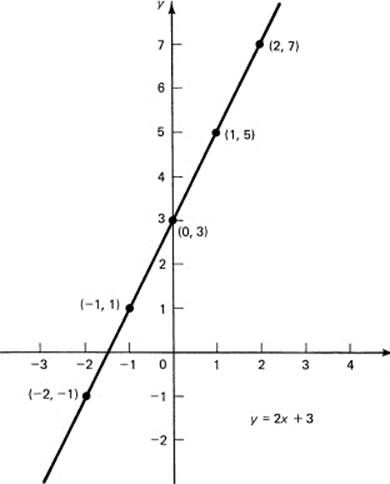
Figure 5.4-1 y = 2x + 3

But it is a characteristic of mathematicians that they have learned not to believe the obvious. Are we sure that all pairs of numbers satisfying the equation will lie on a straight line, and conversely? The picture looks nice and convincing, but some algebra would be more so. How could we convince ourselves of this statement? Never mind that we said that a linear equation corresponds to a straight line. Are you completely sure? What do you know about a straight line? The one thing you surely remember is that a straight line is the shortest distance between two points. How can you use this piece of information (which amounts to the basic definition of a straight line)? A little thought about the very few relevant tools you have available suggests that the triangle inequality is the clue; for a straight line it must be an equality. Therefore, we will pick three distinct points, any three points, on the line. Let them be p₁, p₂, and p₃ with p₂ between the other two. “Between” means, in this case, that the x coordinates of the three points have the “betweenness” property. Of course, we expect that the y coordinates will have the same property.

Given the general linear equation of the form (5.4-1),

the assumption that these three points p₁, p₂, p₃ each lie on the line means that we have the following three equations (the coordinates of each point must separately satisfy the equation if it lies on the line):

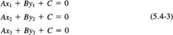
where the point p_i has the coordinates (x_i, y_i). We want to show that

(Remember that p₂ is between p₁ and p₃.) Rather than write out the distance function (5.2-1) for each pair of points, we write a typical distance from p_i to p_j.

If B ≠ 0 (we will take care of the case B = 0 in the next paragraph), then subtract the jth equation of (5.4-3) from the ith equation (note that C cancels out), and divide by B to get

We have, therefore, when we put this into the distance function (5.4-4),

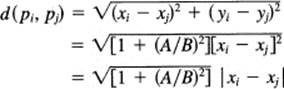
The distance along the line is proportional to the distance between the x coordinates of the points. It is the same constant of proportionality for each pair of points. The distance along the x-axis obeys the triangle inequality trivially; the distance from p₁ to p₂ plus the distance from p₂ to p₃ along a straight line equals the distance from p₁ to p₃ when p₂ is between the other two points. From this it follows that the result is proved, that a linear equation corresponds to a straight line.

The special case of B = 0 (which was earlier set aside) means that the equation is

The only admissible x value is −C/A (assuming that A ≠ 0). The line is a vertical line parallel to the y-axis, since the points (−C/A, y), for any y, all satisfy the equation. The term in x in the distance function drops out, and we have the same argument along the y-axis as we had along the x-axis. Notice that we are in trouble when we have a vertical line; we do not have a function corresponding to the line since functions must be single valued.

The (degenerate) case that both A and B are zero forces C = 0, and we do not have an equation at all. In this degenerate case we have the whole plane; there are no constraints on the coordinates!

A linear equation is a straight line, but does every straight line correspond to a linear equation? Suppose we did have a straight line in the plane. Pick any two distinct points, say p₁ and p₂, on the line (with x₁ ≠ x₂). We can use these two points to find the unique linear equation that passes through them. To actually find the equation of the line, we again use the method of undetermined coefficients. Assume the general form of the Equation (5.4-1),

The coordinates of the two distinct points that lie on this line generate the two equations

To eliminate A from these two equations, we multiply the top equation by − x₂, the second equation by x₁ and add the two equations. We get

If the important quantity, called the discriminant,

then clearly from (5.4-6) C = 0 (unless x₁ = x₂, which is a vertical line). The case C = 0 means that the line has the point (0, 0) on it. This in turn means that the line goes through the origin of the coordinate system. To complete this special case, assume that x₁ ≠ 0. Then the equation involving this point becomes

and putting this in the general form (remember that for this case C = 0) we have, finally,

as the equation through the two points.

If we look at this result, we see how obvious it is. Certainly, the point (0, 0) satisfies the equation (we are now being careless with the words “point” and “coordinates” since we have identified a correspondence between them), and almost as clearly the point (x₁, y_i) satisfies the equation. We could practically write the equation directly from the given conditions.

We now return to the main problem. If the discriminant in (5.4-7) is not zero, that is, if

then we solve for the unknown quantity B:

If we use multipliers on the two original equations (5.4-5) of y₂ and −y₁ and add, we eliminate B. We get, by similar arguments,

Note that the denominator is the same as before (5.4-9). Also note that A and B are both proportional to C, and therefore if C ≠ 0 it can be divided out of each of the three terms of the equation. The equation becomes (when we multiply by the discriminant)

It is easy to check the algebra by noting that the two points p₁ and p₂ both lie on this line. To do this, merely set x = x₁ and y = y₁ and get from (5.4-10)

and all the terms cancel. And similarly for the second point.

There are a couple of special cases to note in our analysis. If the two x values are the same, that is, x₁ = x₂, then the equation is that of a line that is vertical; while if the two y values are the same, then the line is horizontal.

If C = 0, then from (5.4-6) the discriminant equals 0 (or else B = 0, which leaves a degenerate equation Ax = 0), and we have a line through the origin. The condition C = 0 means that there is a linear relation between x and y of the form y = (–A / B)x.

Now consider any other point on the original straight line. Since we proved that a linear equation is a unique straight line, it follows that this point must also be on the line we calculated through the two points. Thus any point on the original line is on the computed line; the line and the equation are in some sense the same thing!

EXERCISES 5.4

1.Verify that the second point lies on the line (5.4-10) we derived above.

Find the line through the two points:

2.(2, –6) and (–1, 1).

3.(6, 4) and (0, 0).

4.(–1, –1) and (–3, –5).

5.Find the equations of the sides of the triangle having vertices (0, 0), (1, 3), and (−2, −3).

6.Draw a diagram of the analysis of this section and include all special cases. Complete the missing arguments.

7.Using Equation (5.4-1), what is the condition that the line be vertical? Be horizontal? Pass through the origin?

8.In Equation (5.4-1), give the geometric meaning of A = 0. Of B = 0. Of C = 0.

5.5 SLOPE

Geometrically speaking, we feel that a straight line has a constant slope, where by the word “slope” we mean the rise that occurs in going from one point p₁ to another (different) point p₂ on the line, divided by the horizontal distance between the two points; that is,

Also, it is said to be “rise over the run.” In mathematical notation, this is

where m is the conventional notation for the slope (see Figure 5.5-1). A horizontal line has zero slope. Notice that if we interchange the two points p₁ and p₂ in the formula (5.5-1) we get the same slope, as we should.

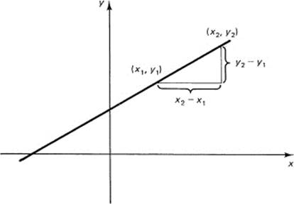
Figure 5.5-1 Slope

Are we sure that the slope of a straight line is independent of the choice of the two points we use? It ought to be, but let us check this algebraically. We have for the general equation of a line

The following two equations represent the fact that the two points p₁ and p₂ lie on the line:

To eliminate C, subtract the second equation from the first:

Divide both sides by B(x₂ − x₁), supposing that it is not zero, and rearrange slightly to get

Thus the slope m depends only on the coefficients A and B and does not depend on the two particular points p₁ and p₂ chosen to compute the slope. Nor does the slope depend on C. Changing the value of C only raises or lowers the line, but does not change the slope of the line.

The slope of m is related to the angle φ (Greek lowercase phi) between the line and the x-axis, as shown in Figure 5.5-2.

Since the line is not usually thought of as having a direction along itself, it is often convenient to limit the angle to a range of 180°. The choice can be –90° < φ ≤ 90°, or 0 ≤ φ < 180°, depending on the needs of the situation. It is convenient to make no general restriction on the angle but let the problem dictate which angles to use.

When the line is vertical, then x₁ = x₂ and there is technically no slope since we cannot divide by zero in form (5.5-4). See Figure 5.5-3 for the corresponding vertical line. It is convenient to say “the slope is infinite,” meaning that there is no finite number to describe the slope.

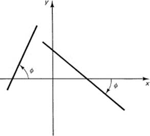
Figure 5.5-2 Angle of line

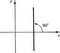
Figure 5.5-3 Infinite slope

We next look at the angle between two lines having slopes m₁ and m₂ (Figure 5.5-4). The angle between them is

To get things in terms of the slopes, we naturally take the tangent of both sides. The trigonometric identity for the tangent of the difference between two angles (16.1-17) is

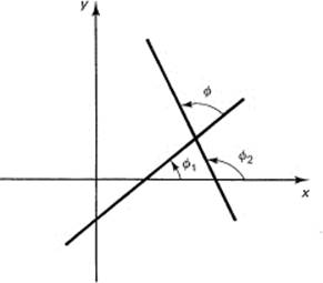
Figure 5.5-4 Angle between two lines

Hence, on substituting the slopes m_i from each line,

Example 5.5-1

Consider the two lines

From Equation (5.5-4) we know that the slope of the line described by the first equation is (solve for y and the slope is the coefficient of x)

For the second equation,

Therefore, the tangent of the angle between the two lines is, using (5.5-6),

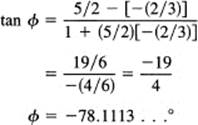
See Figure 5.5-5.

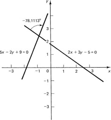
Figure 5.5-5 Angle between two lines

The condition for two lines to be perpendicular is of special interest. We can reason that if ϕ = 90° in (5.5-6) then the tangent is infinite, and hence the denominator on the right-hand side must be zero:

or

The slopes of perpendicular lines are the negative reciprocals of each other. When two lines are perpendicular to each other, they are said to be normal to each other. Note the symmetry in the formulas.

EXERCISES 5.5

What is the slope of the following lines:

1.y = 3x – 6

2.y = –3x + 6

3.x = 2y – 7

4.3x + 2y = 9

5.px + qy = r

6.What is the tangent of the angle between the lines x + y – 1 = 0 and 2x – y = 0?

7.What is the tangent of the angle between the lines 3x – 5y + 7 = 0 and 2x + y = 0?

8.Show that the lines 5x + 7y = 9 and 7x – 5y = 0 are perpendicular.

9.Show that the lines x + y – a = 0 and x – y – b = 0 are perpendicular.

10.What is the slope of a line perpendicular to the line x + 3y = 0?

11.Show by algebra that, if line 1 is perpendicular to line 2, and line 2 is perpendicular to line 3, then line 1 has the same slope as line 3.

12.Show that the perpendicularity condition for two general lines A_ix + B_iy + C_i = 0; (i = 1, 2) is A₁A₂ + B₁B₂ = 0.

5.6 SPECIAL FORMS OF THE STRAIGHT LINE

We have just seen that there is a one-to-one correspondence between straight lines and the general linear equation

In a sense this is all we need to know beyond (1) the definition of the slope of a line (5.5-1)

and (2) the distance between two points, which is given by (5.2-1):

However, straight lines occur so often that it is worth a little time to learn a few special cases.

First, there is the two-point form of the line. Two distinct points determine the slope m of the line by Equation (5.6-2). Next, by inspection we see that the equation

passes through the point (x₁ y₂ and has the right slope. It clearly also passes through the point (x₂, y₂). Of course, the points p_x and p₂ may be interchanged if desired. In this form (5.6-4) the slope must be a finite number; the line cannot be vertical (see Figure 5.6-1). However, if we write Equation (5.6-4) in the more symmetric form by multiplying by the denominator x₂ – x_i9 we get

and this can represent a vertical line (which occurs when x₁ = x₂). In this special case the left-hand side is zero (we assumed that the two points were distinct, so it follows that y₂ ≠ y_i); therefore, we have

x – x₁ = 0

as the equation of the vertical line.

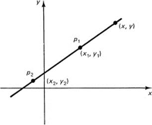
Figure 5.6-1 Two-point form

Second, there is the point-slope formula

which is the same as (5.6-4) with the slope replaced by the letter m (see Figure 5.6-2). Again, the line cannot be vertical in this form.

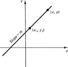
Figure 5.6-2 Point-slope form

Third, there is the slope-intercept form

where b is the intercept on the y-axis (meaning the value of y when x = 0, where the line intercepts the y-axis). It comes from the point-slope formula (5.6-6) by transposing the yi term to the right and combining it with the other term so that b is defined as

b = y₁ + mx₁

An alternative approach is to set y₁ = 0 and mx₁ = b. Again, this line cannot be vertical (see Figure 5.6-3).

Fourth, there is the intercept form of the line

where a is the value of the x intercept and b is the value of the y intercept. The intercept form does not allow for lines through the origin, nor vertical, nor horizontal lines (see Figure 5.6-4).

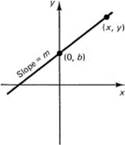
Figure 5.6-3 Slope-intercept form

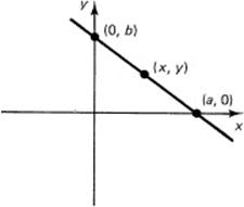
Figure 5.6-4 Intercept form

Example 5.6-1

These examples show how to go from geometric properties to equations. We can illustrate each type easily.

Given the two points p₁ = (2, 3) and p₂ = (4, –2) (see Figure 5.6-5), we get from the two-point form (5.6-4)

which is

Given the point (3, 5) and the slope m = 4, the point-slope formula (5.6-6) gives

y – 5 = 4(x – 3)

Given the slope m = 4 and the y intercept –3, we have, using the slope-intercept Equation (5.6-7),

y = 4x – 3

Finally, given the x intercept 3 and the y intercept –2, we have the line, using (5.6-8),

Multiplying through by 6, we get

2x – 3y = 6

These are some of the ways you can go from geometric properties to equations.

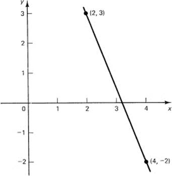
Figure 5.6-5 Two-point line

As a general rule, two conditions are sufficient to determine a line. A condition can be (1) a slope or (2) passing through a point. Note that an intercept is simply a point with one of its coordinates equal to zero. The special forms are merely convenient ways of writing the equation initially or, conversely, having written the equation in that form, of finding the geometric properties of the line. Note that when the special equations are used there can be implied restrictions on the solutions you can find.

Example 5.6-2

These examples show how to go from equations to geometric properties. Given the general line

Ax + By + C = 0

you can assign any value x (unless B = 0), compute a corresponding y, and thus find a point on the line. Suppose B ≠ 0; you can write the above equation in the form

and the above computation is easy. If two points are wanted, then choose a second x value. For plotting purposes it is wise to have the points far apart.

For the slope, you clearly have (from the slope-intercept form)

and the corresponding y intercept (x = 0) is – C/B.

The two intercepts can be found from the general equation by dividing by – C (which must not be zero in this case). You then write the equation in the proper intercept form:

Thus the x intercept is –C/A and the y intercept is –C/B.

An alternative way is to first put x = 0, thus finding the y intercept, b = –C/B, followed by putting y = 0 to get the x intercept, a = –C/A, and finally putting these into the intercept form.

In these ways you can easily pass from the equation to the geometric properties of the line.

Example 5.6-3

Midpoint of a line segment. Find the midpoint of the line segment running from (2, 4) to (–4, 6). A little thought (and a look at Figure 5.6-6) suggests that the coordinates of the midpoint must be the average of the coordinates of the end points:

This immediately suggests the general rule: the midpoint of the line segment from (a, b) to (c, d) has the coordinates

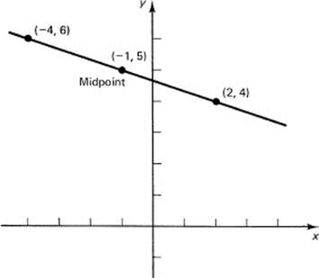
Figure 5.6-6 Midpoint

EXERCISES 5.6

Find the equation through the following points:

1.(2, –3) and (3, –4)

2.(2, 2) and (3, 3)

3.(2, 1) and (5, 1)

4.(–1, 1) and (1, –1)

Find the line through the following:

5.(0, 0) with slope –3.

6.(1, 1) with slope –1.

7.(4, –2) with slope –1.

8.Find the line with intercepts –a and –a. What is the slope?

9.Given the line 3x – 4y = 19, what is the slope? The x intercept?

10.Given the line x + y + 1 =0, what is the slope and the y intercept?

11.Find the intercepts of the line. 2x + 3y + 4 = 0.

12.Find the intercepts of the line. 7x + 9y + 5 = 0.

13.Find the midpoint of the line segment between (–3, 3) and (3, –1).

14.Find the midpoint of the line segment between the points (p, q) and (r, s).

15.Find the formula for the and points of a line segment (trisection).

16.*Generalize Exercise 15.

5.7 ON PROVING GEOMETRIC THEOREMS IN ANALYTIC GEOMETRY

In principle, you can use the analytic geometry approach and prove various theorems in (synthetic) Euclidean geometry, but in fact we use the two methods for different purposes most of the time. There is some overlap, as the following example shows.

Example 5.7-1

Prove that the three perpendicular bisectors of the sides of a triangle meet in one point. Since it is a problem in geometry, the absolute values of the coordinates do not matter; so we can pick the coordinate system to make the algebra as easy for ourselves as possible. This observation suggests we pick the origin of the coordinate system at one of the vertices of the triangle, say A. Next we put the x-axis along one side to the point B, which will now have, say, the coordinates (b, 0). The third vertex, C, will now have coordinates (c, d), which are arbitrary. (See Figure 5.7-1 for one specific arrangement of the points.)

We just saw (Example 5.6-3) that the midpoint of a line segment has coordinates that are the average of the coordinates of the two end points. We now take the sides one at a time and construct the perpendicular bisectors: lines through the midpoints and with the negative reciprocals (5.5-8) of the slopes of the corresponding sides. For the side AB we have the midpoint as (b/2, 0) and the slope m = 0. Hence the perpendicular bisector has the equation

This is a vertical line through the midpoint, and we see that it is correct.

The second side, AC, has the midpoint (c/2, d/2), and the slope of the side is m = d/c. The perpendicular bisector is, therefore, from the point-slope formula (5.6-6),

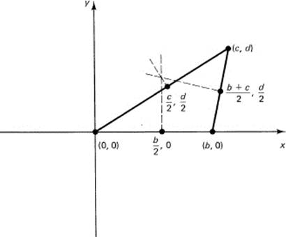
Figure 5.7-1 Perpendicular bisectors

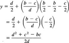
This line intersects the earlier perpendicular bisector x = b/2 at the y value (put x = b/2):

When we simplify this, we get

Thus the intersection of the first two perpendicular bisectors is at the point x = b/2, and y is equal to the above value (5.7-1).

For the third side, BC, we have the midpoint, ((b + c)/2, d/2), and the slope of the side is m = d/(c – b). Hence the perpendicular bisector of this side is given by the equation

This line intersects the first perpendicular bisector at x = b/2, so the corresponding y value is given by

as before (5.7-1). Hence the three perpendicular bisectors have the same common point, and we have proved the theorem.

EXERCISE 5.7

1.Prove that the diagonals of a parallelogram bisect each other. Hint: Find their midpoints.

5.8* THE NORMAL FORM OF THE STRAIGHT LINE

The normal form of the equation is very useful when you are interested in the distance of a point from a given line. From Figure 5.8-1 we see that the distance p from the origin to the line in a perpendicular direction (the shortest distance from the origin to the line) meets the x-axis with an angle θ (theta). What are the intercepts of the line in terms of the distance p? The x intercept a is found from the lower triangle to be

Similarly, from the upper triangle, the y intercept is

Next, using the intercept form of the line (5.6-8),

We have (after some algebra)

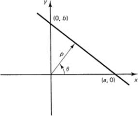
Figure 5.8-1 Normal form

How can we get the general equation of a line (5.5-2) into this form? We note first that

Therefore, if we take the general equation

Ax + By + C = 0

and divide by

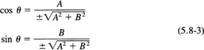
we will have the correct general form, usually called the normal form, where all + or all – signs are used:

How do we decide which sign to use? In the form we have taken (5.8-1), the quantity p is positive. Thus the sign of the square root must be taken to make p positive; that is,

The square root has the opposite sign to that of C: p is positive is the rule.

In this form we make the identification by comparing it with (5.8-1):

From this we get

As a check, we note that the slope of the original line is –A/B and that (5.8-4) is the negative reciprocal, as it should be.

Example 5.8-1

Suppose we have the equation

3x + 4y + 10 = 0

and we want to put this into the normal form. Since A² + B² = 3² + 4² = 5², we divide by ±5. We need to pick the minus sign to make p positive. Thus we divide through by –5 to get the equation

as the normal form (5.8-1) of the equation (see Figure 5.8-2). The distance of the origin from the line is 2. From the sign of the coefficients (sin θ < 0, cos θ < 0), 0 must lie in the third quadrant.

If we hold θ fixed (meaning that the first two coefficients in the normal form are not to be changed) and put into the equation the coordinates of any point p₁ = (x₁, y₁), we will find a new p value for an equation of a line that is parallel to the original given line. It is necessary to distinguish between the subscripted p_x, which is a point, and the distance p of the line from the origin. But p is the perpendicular distance from the line to the origin. The difference between the new p and the old p is exactly how far the point p₁ is from the line (see Figure 5.8-3). The distance of the point from the line can be found directly by simply substituting the coordinates of the point p₁ into the normal form of the line to get

As seen from Figure 5.8-3, this d is the distance of the point from the line. If d > 0, then the point is on the far side of the line from the origin, and if d <0, then it is on the near side.

Thus the normal form is useful for finding the distance from a point to a line.

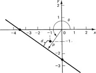
Figure 5.8-2 3x + 4y + 10 = 0

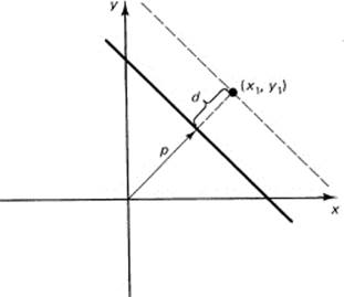
Figure 5.8-3 Distance of a point to a line

Example 5.8-2

Using Example 5.8-1 suppose we find the distance of the point (– 1, – 1) from the line. We have from (5.8-5)

The negative distance clearly means that the point is on the side of the line that includes the origin (Figure 5.8-2).

Example 5.8-3

Angle bisectors. How can we find the bisector of the angle between two lines? We know that the bisecting line is a linear equation and that it goes through the common point of the two given lines. What else do we know about the bisector? Some thought and we recall that any point on the bisector is equidistant from the two sides. This suggests that we put both of the given lines into the normal form and then equate the distances, either both positive or one positive and one negative. The common point of the two sides (the vertex) will, of course, lie on this line. The difference in sign determines which of the two bisectors (Figure 5.8-4) we get. This must give the line we want. First, it is linear and so is a straight line, and, second, we know that any linear combination of two lines must pass through the common intersection; so this must be the bisector of the two given lines.

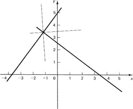
Figure 5.8-4 Bisectors of angles

Example 5.8-4

We illustrate the above with an example. Given the two lines

3x + 4y = 10 and 4x – 3y = –15

we put both in the normal form by dividing by the sum of the squares of the coefficients of x and y. Thus we get the equations

as the two normal forms. The two solutions are therefore

We multiply through by 5 to get rid of the fractions:

from which we get the two equations (use the + and the – signs)

7x + y + 5 = 0 and –x + 7y – 25 = 0

Beware of the fact that in the example both normalizing factors were of size 5; usually they are different. Note: The two bisectors are mutually perpendicular.

EXERCISES 5.8

Put the following equations into normal form:

1.5x + 12y + 36 = 0

2.y = 4x – 5

3.x/3 + y/4 = 1

How far are the following points from the line:

4.(2, 3) and 5x – 12y + 39 = 0

5.(1, 1) and 3x + 3y = 6

6.(1, –1) and x + y = 1

7.Find the tan θ and p for the equation 2x + 2y = 17.

8.*Develop the general equations for the bisectors of two general lines, A₁x + B₁y + C₁ = 0 and A₂x + B₂y + C₂ = 0

9.*Prove that the bisectors of the angles of a triangle meet in a common point. Hint: Pick the coordinates as in Example 5.7-1.

10.*Discuss the normal form of the line when the line passes through the origin.

5.9 TRANSLATION OF THE COORDINATE AXES

To eliminate some terms in an equation, it is frequently very convenient to translate the origin of the coordinate axes to some new point in the plane. Conventionally, this new origin is assigned the coordinates (h, k) in the old coordinate system. Figure 5.9-1 shows such a shift. The values of h and k are shown in the picture as being positive, but they may be of either sign or zero. Let the new coordinate system use coordinates (x′, y′). Then it is easy to see that

If we solve for the new coordinates in terms of the old, we have

Note the structure of Equations (5.9-1) and (5.9-2).

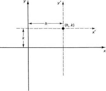
Figure 5.9-1 Translation of coordinates

Example 5.9-1

Suppose we have the line

y = 3x – 7

and wish to shift the origin of the coordinate system to the point (1, –2). We have, using (5.9-1),

y′ – 2 = 3(x′ + 1) – 7

or

y′ = 3x′ – 2

Notice that, of course, the slope m = 3 stays the same.

EXERCISES 5.9

1.Translate the equations x – y – 2 = 0and x + y – 6 = 0 to the coordinate system with the origin at (4, 2).

2.Translate the general equation Ax + By + C = 0 to the point (h, k).

3.Translate the origin of the coordinate system to the common point of the two lines 3x + 4y = 5 and x – y = –5.

4.Develop the theory for translating the origin of the coordinate system to the common point of two arbitrary lines, A₁x + B₁y + C₁ = 0 and A₂x + B₂y + C₂ = 0.

5.Discuss the fact that the translation x = x′ + h followed by the translation x″ = x′ – h leaves the equation unchanged.

6.Discuss the result of one translation followed by another translation.

5.10* THE AREA OF A TRIANGLE

Case Study 5.10-1

Area of a triangle. A common problem in geometry is to find the area of a triangle. Usually the triangle is defined by the three vertices, although the equations of the three sides might be given instead. If the triangle is in the form of three equations, solving the equations two at a time to find the vertices (the common point of the two lines) reduces the problem to the first form, given three points.

The problem looks new, so let us start by doing the simplest case we can imagine, a standard method of approaching problems in mathematics. (See Section 1.5, Hilbert.) Put the first point at the origin, the second point at (x₂, 0) on the x-axis, and the third point at (x₃, y₃). (We do not pick the coordinates a, b, and c as before because we must end up with three general points with general coordinates.) We look at the picture, Figure 5.10-1. The area A is the base, x₂, times the altitude, y₃, times ; that is

and we have the answer.

Next, we approach nearer to the general case by moving the point (x₂, 0) off the x-axis to the general point (x₂, y₂) (see Figure 5.10-2). In this figure the area of the shaded triangle (which is what we want) is the difference between the areas of the two triangles, both with the same base a on the Jt-axis. Thus the area is now

where a is the x intercept of the line passing through the third and second points.

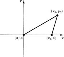
Figure 5.10-1

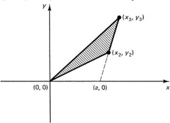
Figure 5.10-2

To find this intercept a, we first find the line through the points p₃ and p₂. We begin by finding the slope (5.5-1)

Then we use the point-slope formula (5.6-6)

y – y₂ = m(x – x₂)

Where does this line cross the x-axis? At y = 0. Therefore, the solution x is our a value (meaning set y = 0 and x = a). We have

– y₂ = m(a – x₂)

Now divide both sides by the slope m and then eliminate m using the slope formula above (5.10-3) to get

Solve for a by transposing x₂ and getting a common denominator:

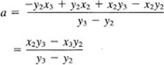
Now put this value of a into the earlier formula (5.10-2) for the area. We get

The final step in deriving the general formula for the area is to translate the axis to the point (–x₁, –y₁ using (5.8-1) so that in the new coordinate system the point that was at the origin will now have coordinates (x₁, y₁). Dropping, for the moment, the factor, we have

x₂y₃ – x₃y₂ = (x′₂ – x₁)(y′₃ – y₁) – (x′₃ – x₁)(y′₂ – y₁)

Expand the right-hand side and drop the primes for convenience:

= x₂y₃ – x₂y₁ – x₁y₃ + x₁y₁ – x₃y₂ + x₃y₁ + x₁y₂ – x₁y₁

The x₁y₁ terms cancel, and rearranging the terms as well as including the factor we get, finally, for the area of the general triangle

The symmetry of this formula is highly appealing. For those who know determinants, this can be written in the form of a determinant

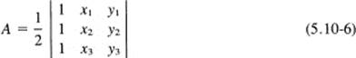
The area will turn out to be positive if the points are taken in a counterclockwise direction and negative if in the clockwise direction. We will later see why we might want to admit negative areas.

The formula passes some tests of reasonableness.

1.If any two points are the same, then the area is 0.

2.As noted, there is a high degree of symmetry in the formula. Thus, if the names of the points are rotated, 1 to 2, 2 to 3, and 3 to 1, the area (and formula) stays the same. And similarly for a rotation of the point labels in the reverse direction.

3.We can verify the formula in a special case to see if the front coefficient is correct. The case (0, 0), (1, 0), and (0, 1) checks this. We get

as it should.

4.We can also try a second special case, x₁ = 0 and y₁ = 0. The result agrees with our preliminary formula (5.10-4):

Rule: Whenever you derive a general formula, it is wise to subject it to a number of specific tests as well as general ones, such as having the necessary symmetry and invariance. While no number of specific tests will prove the formula correct for all cases, usually you can find a set that will greatly increase your confidence in the result. Of course, checking all the reasoning and all the algebra is one test; but, unfortunately, if you have made an error in the derivation, you are apt to make the same one again!

EXERCISES 5.10

Find the area of the triangle having the following vertices:

1.(1, 0), (0, 1), and (1, 1)

2.(1, 2), (2, 3), and (–3, –2)

3.(a, a), (b, b), and (c, –c)

4.(a, b), (b, c), and (c, –a)

5.Using (5.10-5), translate the x coordinate an amount h. Note the invariance of the area. Do the same for the y coordinate.

5.11* A PROBLEM IN COMPUTER GRAPHICS

A problem that occurs constantly in computer graphics is the “hidden point problem.” You are often given the coordinates of the vertices of the various figures whose sides are straight lines, and are asked to show what is seen and what is hidden from some viewpoint. For convenience we first translate the viewpoint to the origin.

Case Study 5.11-1

Hidden point. To decide if a point is in front of an object or behind it (Figure 5.11-1), we need first to find the equation of the line through the given pair of points that define that edge, imagine the equation in normal form, and substitute the coordinates of the point into the line. We do not actually need to find the distances, only the sign. Therefore, there is no need to find the squares and the square root; it is only necessary to get the sign of the constant term correct, substitute the coordinates of the point into the equation, and note the resulting sign.

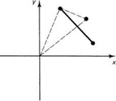
Figure 5.11-1 Hidden point

To decide if some point is to the right or left of another point, we can merely use the area formula. With the viewpoint put at (0, 0), we have the simple formula

2A = x₂y₃ – x₃y₂

Again, it is only the sign that we want, not the actual angles involved. We must test, of course, that the hidden point is between the ends of the line segment.

These two observations, based on a slight knowledge of analytic geometry, together with the belief that one should not compute more than is necessary, is all that is needed to solve this common computer graphics problem. Neither the actual distances nor the actual angles are needed in many cases, only whether or not some point is visible. In this geometry, it is not the distances that matter, only in front or behind, nor the angles, only to the right or to the left. Both are easily solved using the elements of analytic geometry and greatly decrease the computer time used to solve the hidden point problem.

EXERCISES 5.11

1.Given the line segment from (1, 1) to (3, –4), give the details for finding if the point (x, y) is hidden by the segment or not.

2.*Given the four vertices of a quadrilateral, p₁, p₂, p₃, and p₄ in a counterclockwise order, and a general point (x, y), indicate the main steps you would use to decide if the point (x, y) is inside or outside the quadrilateral. (Beware of the origin’s being inside the quadrilateral.)

5.12 THE COMPLEX PLANE

A complex number of the form a + ib (i = ) has two real numbers, a and b, and this suggests plotting a complex number on a plane similar to the Cartesian plane except that we use the axes x and iy.

Example 5.12-1

Plot 2 + 3i, –2 – 3i. See Figure 5.12-1.

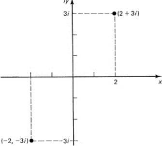
Figure 5.12-1 Complex plane

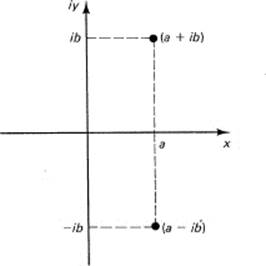
Figure 5.12-2 Conjugate points

Example 5.12-2

Plot the complex conjugate points a + ib and a – ib. See Figure 5.12-2.

The absolute value squared of a complex number is the product of the number and its conjugate (4.8-8):

Thus the absolute value plays a role in the complex Argand (1768–1822) plane similar to the Pythagorean distance in the Euclidean plane. The absolute value of a complex number is the modulus of the number, (4.8-7), and plays the role of the distance from the origin.

The representation of complex numbers in the complex plane gives a natural picture of the numbers, and hence tends to give the student a feeling that complex numbers are less strange than when only the algebraic i = is used. Together with the distance function, which is the absolute value, the Argand plane seems to provide some reasonableness to complex numbers.

For example, when two complex numbers are added, say a + ib and c + id, their sum

is represented by the diagonal of the parallelogram with the two sides a + ib and c + id, as shown in Figure 5.12-3.

From Figure 5.12-4 we see that

The modulus of x + iy is therefore

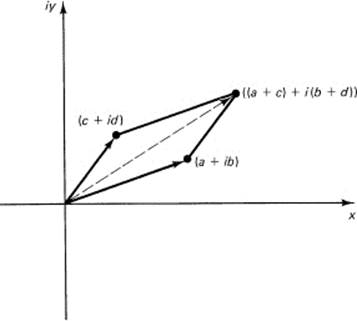
Figure 5.12-3 Additional of complex numbers

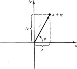
Figure 5.12-4

Some of the power of complex numbers arises from the simple observation that a single equation in complex numbers is equivalent to two real equations, since a complex number a + ib = 0 requires both a = 0 and b = 0. There are also many interesting relationships that are best understood when written in the form of complex numbers, and we will see many of them in this book. Trigonometry is especially given some unity when complex numbers are used; it is no longer a miscellaneous collection of random formulas (see Section 21.5).

The Euclidean (Cartesian) plane and the complex (Argand) plane are different. In the Euclidean plane a pair of real numbers (x, y) are used to name a point; in the complex plane a single complex number x + iy defines the point.

EXERCISES 5.12

1.Plot the points 3 + 3i and 3 – i.

2.Find the modulus of 3 + 4i.

3.Show that

4.For real a, show that |(ai – 1)/(ai + 1)| = 1

5.Find the modulus of 1/(1 + i).

6.Show that |cos x + i sin x| = 1.

7.Give the modulus of i, –i, 1, –1.

8.Prove that the modulus of a complex number and its conjungate are the same.

9.Prove that the |x|² = |x²|.

10.Prove |x||y| = |xy|, where x and y are complex numbers.

11.Generalize Exercise 3 and contrast with Exercise 8.

5.13 SUMMARY

You have begun the topic of analytic geometry. The basic idea of analytic geometry is that there is an exact correspondence between number pairs (x, y) and points in the plane. Therefore, there is a correspondence between parts of algebra and geometry. You have also seen that the simplest geometric curves (straight lines) correspond to the simplest algebraic equations (linear equations). You have further learned how to go from geometric properties of straight lines to linear algebraic equations and back again to geometric properties. Finally, you learned how to translate the coordinate system from one origin to another. Along the way you found how to compute various useful things such as the distance between two points, the slope of a line, angles between lines, intersections of lines, the distance of a point from a line, and the area of a triangle. You have also used such things as the method of undetermined coefficients, the solution of simultaneous equations, some elements of trigonometry, and others.

We also continued your introduction to complex numbers beyond the usually brief treatment when you first see the quadratic equation. In beginning algebra, complex numbers are used only to explain where the two real roots disappear when the discriminant b² – 4ac passes from positive to negative values. Plotting complex numbers in the Argand diagram provides one means of grasping what role they play in mathematics. The complex plane is one of the major tools in advanced mathematics, both continuous and discrete, as well as in many applications in the real world, such as unifying electric and magnetic phenomena.