Methods of Mathematics Applied to Calculus, Probability, and Statistics (1985)
Part I. ALGEBRA AND ANALYTIC GEOMETRY
Chapter 6. Curves of Second Degree—Conics
6.1 STRATEGY
In the previous chapter we examined linear equations and found that they correspond to straight lines and, conversely, that straight lines correspond to linear equations. It is natural to turn next to the general quadratic (second degree) equation. However, it is sound strategy to approach the subject cautiously and begin with simple things. The simplest geometric figures, after straight lines, are circles, which we examine first. They will turn out to be particularly simple quadratic equations. Then we will gradually examine more complex quadratic equations until we have reached the general case. This is the way new territory is generally explored; the easier cases are tried first so you can get oriented, and when the easy cases are done you are ready to complete a general survey of quadratic equations (see Section 1.5, Hilbert).
6.2 CIRCLES
Consider a circle centered about the origin. From the definition of a circle, all the points on the circumference are at a fixed distance from the origin. That is, any point with coordinates (x, y) on the circle must satisfy the distance condition (5.2-1) from the origin.
x2 + y2 = r2
where r is the radius of the circle. For example,
x2 + y2 = 25
is a circle of radius 5 centered about the origin.
There is an ambiguity in the common use of the word “circle.” We say, “Draw a circle” and clearly mean draw the circumference. But we also speak of the area of a circle, meaning everything inside. To describe the set of points, we can say that the circumference is the set of points satisfying
x2 + y2 = r2
The circumference plus the inside is the set of points satisfying
x2 + y2 ≤ r2
Finally, the set of points satisfying
x2 + y2 < r2
is the inside of the circle.
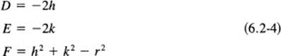
If you want the center of the circle to be at some other point than the origin, say at the general point (h, k), then the equation is
![]()
which describes all points a distance r from the center (h, k). We can either find the equation directly from the definition of the distance, or else we can use the equation of the circle about the origin and translate the origin to the new center (Section 5.9). Notice that these equations are not single-valued functions.
Example 6.2-1
The circle about the point (3, 4) of radius 5 is (see Figure 6.2-1)
(x – 3)2 + (y – 4)2 = 25
This can also be written in the form (expand the two square terms)
x2 + y2 – 6x – 8y = 0
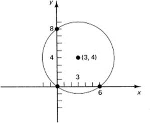
Figure 6.2-1 Circle centered at (3, 4)
Thinking about this particular circle, we see that it should pass through the origin (since the center is exactly 5 units from the origin and 5 is also the radius). To check this, we simply put in the coordinates (0, 0) and then note that they satisfy the equation.
The general circle (6.2-1) of radius r about the point (h, k) can be written in the expanded form
![]()
which takes the general form
![]()
The reason for the choice of the letters D, E, and F will become apparent later. Of course, this equation could be multiplied through by any nonzero constant, and it would still have the same points as solutions of the equation. Indeed, any of the equations (6.2-1), (6.2-2), or (6.2-3) when multiplied by a nonzero constant represents the same circle. It is conventional to pick the coefficient of x2 + y2 as 1.
A comparison of the coefficients of the two forms (6.2-3) and (6.2-2), the algebraic and the geometric, shows that they are related by the conditions
We now know how to go from the definition of a circle of given center and radius to the equation for a circle. Can we handle other given conditions?
Suppose you are given three points to determine the circle. How will you find the corresponding equation? Easy! Use the method of undetermined coefficients. Because there are only three parameters, we have only to impose the three conditions that the three points lie on the circle when you write it in the general form (6.2-3). Since the general form has three parameters, D, E, and F, you will find that you have three linear equations to solve for the three parameters.
Example 6.2-2
In this first example we pick the points to make the algebra and arithmetic easy. Suppose the three points are (0, 0), (6, 0), and (0, 8). Using the form (6.2-3), these three points will generate the three equations (see Figure 6.2-1)
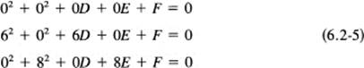
Note that these are linear equations in the unknown coefficients D, E, and F and are therefore comparatively easy to solve.
From the top equation, F = 0. From the second equation, D = –6. And from the third equation, E = – 8. Thus we have the equation of the circle through the three points
![]()
It is easy to check that each of the original points lies on the circle (the coordinates of the points satisfy the equation).
Generally, three given points will not allow such an arithmetically simple solution of the three equations, but the method is the same. The method of undetermined coefficients wil always lead, for circles through three points, to three linear equations in the three unknowns D, E, and F. These three equations can generally be solved for the D, E, and F which define the circle algebraically. The only exception when these three equations cannot be solved for the unknowns is the case when the three points fall on a straight line (see Exercise 6.2-11).
You can now see some of the power of the method of undetermined coefficients as it applies to analytic geometry—assume the general form and apply the conditions to determine the unknown coefficients.
Example 6.2-3
As an example where the algebra is slightly more difficult, but still in terms of nice integers, consider the circle through the three points (1, 1), (–1, 1), and (2, 3) (Figure 6.2-2). Put these coordinates into the general form for a circle, Equation (6.2-3):
x2 + y2 + Dx + Ey + F = 0
and get the three equations corresponding to Equations (6.2-5)
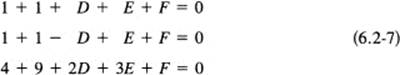
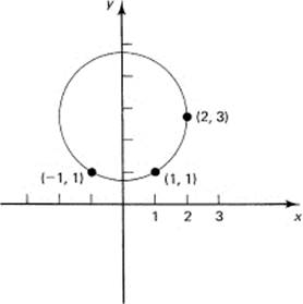
Figure 6.2-2 Circle through three points
Next rewrite these in the conventional form, with the unknowns on the left-hand side and the constants on the right:
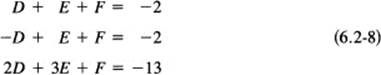
To use what little symmetry we have, we subtract the second equation from the first, which eliminates the E and F terms. We get the simple equation
2D = 0
which implies that D = 0. We drop one of the two equations we used, say the first equation. The lower two equations of (6.2-8) are now
![]()
We subtract the top of these two equations from the lower to eliminate the F term, and we get
2E = – 11
from which it follows that
![]()
Substitute this value of E into the top (or bottom) equation of the pair (6.2-9) to get
![]()
Thus the equation for the circle through the three points is
![]()
It is easy to check that Equation (6.2-10) is satisfied by the coordinates of the three points.
Example 6.2-4
Show that the angle in a semicircle (see Figure 6.2-3) is a right angle. We pick the circle as
![]()
and the point on the circle as
![]()
with the semicircle above the y = 0 axis. The slopes of the lines from this point (6.2-12) to the ends of the diameter (–a, 0) and (a, 0) are
![]()
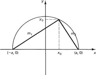
Figure 6.2-3 Angle in a semicircle
The condition for perpendicularity is, from (5.5-7),
m1m2 = – 1
This becomes
![]()
We simplify this to
![]()
which, by (6.2-11), is true since the point lies on the circle. These steps are reversible; therefore, we have shown that the two lines are perpendicular at the point where they intersect the circumference of the semicircle, as required.
These are examples of going from the geometry of the problem to the algebra. We see again the power of the method of undetermined coefficients: you assume the general form and impose the conditions to determine the unknown parameters. It is a powerful, general method in many areas of mathematics.
EXERCISES 6.2
Find the circle given:
1.Center (–1, 1) and radius 1
2.Center (–3, –4) and radius 5
3.Center (1, 1) and radius 2
Find the circles through the following points:
4.(1, 1), (1, –1), (–1, –1)
5.(2, 3), (3, 4), (4, 5)
6.(5, 12), (0, 0), and radius 6 ![]()
7.(0, 0), (0, 10), (5, 13)
8.(1, 10), (1, –1), and radius 4
9.(6, 6), (–6, 6), and r = 2
10.Show that, if (a, b) lies on the circle x2 + y2 = r2, then the points (a, –b), (–a, b), and (–a, –b) also lie on the circle.
11.*If the three points you select to fit a circle to happen to lie on a straight line, what happens?
6.3 COMPLETING THE SQUARE
We next examine problems involved in going from the algebra to the geometry. Suppose we have the equation of a circle and want to determine the geometric properties, the center and radius. How can we do this? We compare the expanded general form (6.2-2) about the point (h, k),
![]()
with the general form (6.2-3),
![]()
We see as before, in Equation (6.2-4), that we must have
![]()
We have only to solve for h, k, and r. Note that it is not a sure thing that we can solve for r, since it might turn out that
![]()
is a negative number (and you can see that if we persisted then we would have a circle with an imaginary radius!).
Since it is a common problem to find the geometric properties, the h, k, and r in this case, from the algebraic equation, we look at a second approach [who wants to remember the formulas (6.3-3)?]. We try to write the general form, Equation (6.3-2),
x2 + y2 + Dx + Ey + F = 0
in the particular form (6.3-1):
(x – h)2 + (y – k)2 = r2
This approach requires you to take the x terms,
x2 + Dx
and get them into the form
(x – h)2
To do this, we complete the square by adding to both sides of the equation
![]()
(in words, add the square of one half of the x term coefficient to both sides). Now we can write (on the left side)
![]()
Similarly, for the y terms we add (E/2)2 to both sides. We get on the left-hand side
![]()
We take the remaining term F of (6.3-2) to the right-hand side, and as a result we have on the right side [see Equation (6.3-4)]
![]()
Therefore, the equation of the circle is
![]()
As before, only if this right-hand side is nonnegative can we have a circle that is real. If it is exactly zero, then the circle is a point at (–D/2, –E/2). If it is positive, then the center of the circle and radius are given by
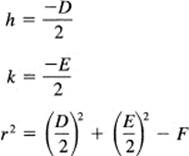
as before. We have derived Equations (6.3-3) by a simple method that is worth learning carefully.
Example 6.3-1
Given the equation
x2 + y2 + 2x – y – 5 = 0
find the center and radius. Transpose the constant term, and complete the square in both x and y (remembering to add the same quantities to both sides to preserve the equality):
![]()
or
![]()
Thus the center is at (–1, ![]() ) and the radius is
) and the radius is ![]() .
.
Completing the square is a very common process in mathematics and is not confined merely to problems involving coordinate changes.
Example 6.3-2
Roots of a quadratic equation. The process of completing the square is exactly what you used when you found the general solution of the quadratic equation in beginning algebra:
![]()
First, you transposed the constant term c to the other side and then divided through by a.
![]()
Next, you completed the square by adding to both sides the square of one-half the x term coefficient:
![]()
Then you found the common denominator on the right-hand side and took the square root to get, after transposing the b/2a term,
![]()
as the final formula. Conventionally, this is written with a single denominator:
![]()
This is the standard formula for the roots of a quadratic, which we have already used several times. It is important to master both the method and the formula for the roots of a quadratic.
Example 6.3-3
Find the two lines through a given point tangent to a given circle. In such a problem we have the freedom to pick the coordinate system as we please, and it is natural to pick the circle centered about the origin. We pick the scale so that the radius of the circle is a; that is, we let the circle be
![]()
We next pick the equation of the tangent line in a convenient form. Since the circle has rotational symmetry, we are not giving up any generality by picking the point at the place x = 0, y = b. Let us take the slope-intercept form (Figure 6.3-1)
y = mx + b
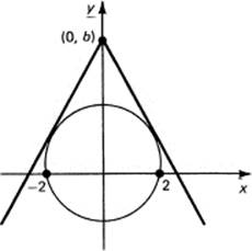
Figure 6.3.1 Tangent lines
What do we mean by the word “tangent”? We mean that the two potential intersections between the circle and the line are actually a single real point. This means that the roots of the quadratic equation, when we have eliminated one variable, say y, will be double. Using (6.3-6), this means that the discriminant b2 – 4ac = 0. To follow this plan, we first eliminate y from (6.3-7) to get the quadratic equation
x2 + (mx + b)2 = a2
which is
(1 + m2)x2 + 2mbx + (b2 – a2) = 0
This quadratic equation has a double root if the discriminant of the quadratic is zero, that is, if
(2mb2) – 4(1 + m2)(b2 – a2) = 0
After some algebra,
4m2b2 – 4b2 + 4a2 – 4m2b2 + 4m2a2 = 0
and canceling the like terms 4m2b2, this comes down to
![]()
Now, taking the square root gives the two slopes (of opposite sign).
![]()
We now have both m and b for the tangent lines.
What is the meaning of the situation when b2 is less than a2? The answer is that the intercept b is inside the circle and the tangent lines are imaginary!
We apparently have mastered the circle and the art of completing the square. For a circle we now know how to go (1) from the geometry to the equation, and (2) from the equation to the geometry. These are the two fundamental steps in analytic geometry.
When we have completed the square for both x and y, we have the equation in the form
(x – h)2 + (y – k)2 = r2
If we choose, we can translate the circle to the origin by the transformation of coordinates (see Section 5.9)
x′ = x – h
y′ = y – k
This transformation can be looked at in two ways. We can think of the coordinates being translated from the origin (0, 0) to the center of the circle, or else we can think of the circle being translated to the origin. The first is called alias, meaning we have the same circle but under a different name. The second is called alibi, meaning not being there (which is the technical use of the word alibi). It does not matter which view you take of the transformation so long as you keep a consistent view. It is when you mix the two (alias and alibi) in the same problem that confusions can arise.
EXERCISES 6.3
1.Complete the square for x2 + 6x.
2.Complete the square for 3x2 + 9x.
3.Complete the square for 5x2 – 3x.
4.Is the point (2, 2) inside or outside the circle x2 + y2 = 5.
5.Find the equation of a circle of radius 7 and center (−2, −3).
6.Find the circle of radius 13 about the center (–5, 12). Show that it passes through the origin.
7.Given the equation
x2 + y2 + 4x – 6y + F = 0
what is the value of F so that the equation represents a point?
8.Find the circle through the points (1, 1), (2, 2), and (3, –3). Give both center and radius. Check by making a drawing of the geometric problem.
9.The British often write the general quadratic as
Ax2 + 2Bx + C = 0
Derive the corresponding formula for the roots. Discuss the amount of arithmetic needed in the two cases to compute the roots from the formulas.
10.Discuss the use of the general form for the circle
x2 + y2 + 2Dx + 2Ey + F = 0
in place of the one we used.
11.Given two intersecting circles
x2 + y2 + D1x + E1y + F1 = 0
x2 + y2 + D2x + E2y + F2 = 0
subtract the two equations to get the equation of a straight line. Describe geometrically what this line must be. Ans.: The line through the two common points of the circle.
12.Given the equations in Exercise 11, multiply one by a constant K and add to the other. Describe what this circle is geometrically. Ans.: A circle through the two common points, and when K = –1 it is a straight line (as in Exercise 11).
13.*Find the tangents to the circle x2 + y2 = a2 going through the point (b, b) (b > 0).
14.*In Example 6.3-3, discuss the case when a = b.
6.4 A MORE GENERAL FORM OF THE SECOND-DEGREE EQUATION
For a circle the coefficients of both the square terms are the same, and it is taken conveniently to be 1. More generally, but not completely general as yet (we are still omitting the cross product term xy), we examine the quadratic form
![]()
We are for the moment assuming that neither A nor C is zero (AC ≠ 0). The cases when AC = 0 will be examined later.
It is natural to complete the square to eliminate the linear terms Dx and Ey. We have, at the first stage of the algebra,
![]()
Notice that we must factor out the leading coefficient of each variable before we start. To complete the squares, we add A (D/2A)2 and C (E/2C)2 to both sides (notice that the leading coefficient must be remembered for each term):
![]()
Next, we translate the coordinate system to “clean up” the equations a bit. Set
which gives
A(x′)2 + C(y′)2 = K
We now drop the primes and divide by K (the case K = 0 will be taken up later):
![]()
Divide the numerator and denominator of the first term by A and of the second term by C:
![]()
To get the expression in a symmetric form, we write the denominators as squares.
![]()
We then have the standard reduced form
![]()
In this form we see the advantage of choosing the quantities as squares of numbers: we have a natural homogeneity in the terms. Had we not done so, then as we moved forward we would have found a great many square roots and would have finally decided to back up and introduce the above notation.
EXERCISES 6.4
Reduce the following to standard form:
1.x2 + y2 + 4x – 6y – 3 = 0
2.3x2 + 4y2 + 2x – 8y + 4 = 0
3.x2 – 4y2 – 4x – 8y – 9 = 0
4.x2 + x + y2 – y = ![]()
5.2x2 + 8x – 3y2 + 12y = 10
6.Find the quadratic (6.4-1) through the four points (0, 0), (0, 2), (3, 1), (1, 3). Hint: Substitute the four points into the general form for the quadratic (6.4-1) (which has essentially four parameters) and solve for the unknown coefficients. One coefficient can be divided out.
7.*Given two general quadratics of the general form 6.4-1, show that any linear combination of them is a quadratic (possibly degenerate) through the common points.
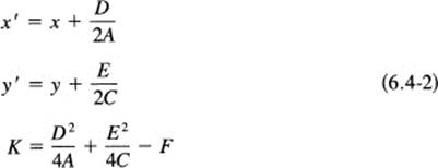
6.5 ELLIPSES
First, we consider the standard reduced form (6.4-4) for the case when both signs are positive. For the moment, assume that a > b > 0. A plot of selected points on the curve gives a shape like that in Figure 6.5-1. It is called an ellipse. We see that the axis crossings (intercepts) are ± a on the x-axis and ± b on the y-axis. Since x and – x always lead to the same y, there is symmetry about the y-axis. Similarly, the presence of only even powers of y means that y and – y lead to the same x, and there is symmetry about the x-axis.
If a = b, then we clearly have a circle of radius a. The ellipses (for b < a) are simply circles shortened in the y direction by the ratio b/a. As you can see by a little thought, an ellipse is the shadow of a circle on a plane when one or the other is tilted with respect to the direction of a parallel beam of light. To sketch the ellipse, we simply draw the box shown in dotted lines in Figure 6.5-1, and sketch the ellipse inside the box. If b > a, then the long direction is up the y-axis.
To get the sketch of the original equation, we merely shift the coordinate axes back to the original ones via the translation equations (6.4-2).
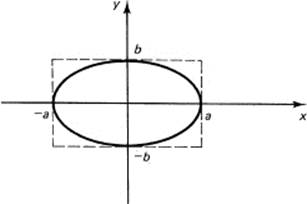
Figure 6.5-1 An ellipse
Example 6.5-1
Consider the equation
![]()
Complete the square and transpose all other terms to the right-hand side:
![]()
Now divide through by 36:
![]()
From this you see that the center of the ellipse is (–1, 2), a = 3, and b = 2. Thus, starting from the equation, you have found the geometrical properties. Figure 6.5-2 shows a sketch of this ellipse.
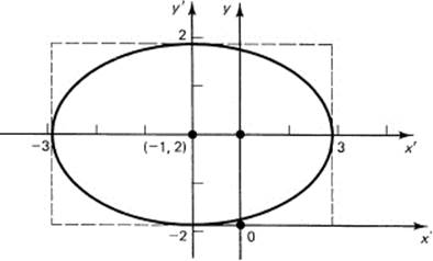
Figure 6.5-2
It is natural to ask, “How can we describe the shape of an ellipse?” Clearly, the values of a and b give the fundamental answer, but they depend on the size of the ellipse and we want to describe the shape. One way is to simply take the ratio of b to a (where we are assuming, as is natural, that both a and b are positive). Thus one measure is the ratio
![]()
In the above example, a = 3 and b = 2, so the ratio is ![]() .
.
The most commonly used measure is, however, called the eccentricity, and is labeled by e:
![]()
where it is assumed that a is greater than or equal to b (if not, you would naturally interchange the roles of a and b even for the ratio, since the shape does not depend on which direction the larger “diameter” of the ellipse lies). In the above example you have
![]()
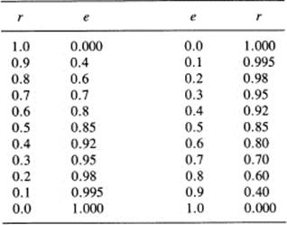
When a = b, you have a circle whose eccentricity e = 0, while the ratio r = 1. Table 6.5-1 demonstrates the relationship of r and e.
Note that the eccentricity e measures small departures from circular better than does the ratio r. We have
![]()
as the direct relationship between the two measures.
Notice that in both measures, e and r, the quantity is independent of the size (the units of measurement) of the ellipse. Such quantities are called dimensionless since they do not depend on the particular units (centimeters or inches) used to measure the dimension. Dimensionless quantities play a fundamental role in science. For example, in (6.4-1), by picking a2 and b2 we made the form dimensionless when the quantities a, b, x, and y are measured in the same quantities.
TABLE 6.5-1
EXERCISES 6.5
Sketch the ellipse for the following:
1.x2/32 + y2/42 = 1
2.x2 + 4y2 = 16
3.x2/42 + y2 = 1
4.x2 + 4y2 – 2x + 8y + 5 = 0
5.9x2 + 4y2 + 36x – 8y + 4 = 0
6.Find the ellipse through the points (0, 0), (0, 2), (3, 1), and (–3, 1).
7.Discuss the ellipse x2/a2 + y2/b2 = k as k goes from 1 through 0 to – 1.
6.6 HYPERBOLAS
The next case we take up has opposite signs on the two square terms in the reduced form (AC < 0). Consider first the case when we have
![]()
The value y = 0 gives x = ± a. As x and y both get large, the size of the two terms on the left becomes very large with respect to the number 1 on the right-hand side. The terms approach each other in size, although, of course, their difference must be 1. We are making a small change in the values of x and y when we replace (for large x and y) Equation (6.6-1) by the equation
![]()
This equation factors into
![]()
Since a product is zero only if one (or both) of the factors is zero, we conclude that we have the two separate straight lines, called the asymptotes of the curve,
![]()
The curves of the hyperbola approach the asymptotes as x and y become large. In Figure 6.6-1 we see the same box as before in dashed lines with dimensions a and b. The two asymptotes go through the comers as shown. We have the vertices of the hyperbola at (±a, 0) and can sketch the curve fairly easily.
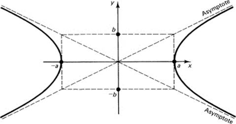
Figure 6.6-1 Hyperbola
If the first term is negative and the second is positive,
![]()
then the vertices are clearly (0, ± b). The asymptotes are the same as before, but the hyperbola goes up the y-axis rather than along the x-axis (Figure 6.6-2).
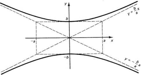
Figure 6.6-2 Hyperbola
Example 6.6-1
To sketch the hyperbola
x2 – y2 + 2x – 6y + 1 = 0
we first complete the square
(x + 1)2 – (y + 3)2 = 1 – 9 – 1 = –9
Next we shift the coordinates and rearrange in conventional form:
(x′)2 – (y′)2 = – 9
Drop the primes, and divide through by the minus 9:
![]()
This hyperbola has vertices (0, ±3) and therefore goes up the y-axis (see Figure 6.6-3). The sketched box is the same for both ellipses and hyperbolas. The difference is that the ellipse lies wholely inside the box, and the hyperbola lies outside. The diagonals of the box provide the asymptotes for the hyperbola, and then you fix the vertices, whether on the x- or on the y-axis (either by trial and error or by remembering that it is the term with the plus sign that gives the vertices).
In terms of the Argand plane, there is an interesting relationship between the ellipse and the hyperbola. The ellipse is described by the equation
![]()
If we write this equation as
![]()
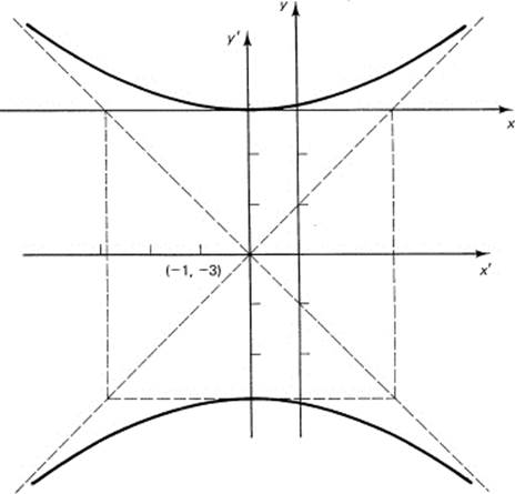
Figure 6.6-3
the result is a hyperbola in the (x, iy) coordinates. Thus what in the Cartesian plane is an ellipse becomes in the Argand plane a hyperbola!
EXERCISES 6.6
1.Plot x2 – y2 + 1 = 0.
2.Plot 4x2 – 9y2 = 36.
3.Plot –4x2 + 9y2 = 36.
4.Plot x2 – y2 + 4x – 6y = 3.
5.Plot x2 + 4x – y2 + 4 = 0.
6.Discuss the hyperbola x2/a2 – y2/b2 = k as k goes from 1 through 0 to –1.
7.Discuss hyperbolas in the Argand plane.
6.7 PARABOLAS
In the general quadratic form, Equation (6.4-1), it is possible that one of the square terms is missing. This is expressed mathematically by AC = 0. Suppose that it is the y2 term that is missing (C = 0). We have, therefore, the form
Ax2 + Dx + Ey + F = 0
to analyze. First, complete the square on x.
![]()
Note again the necessity to factor out the A and to remember it when adding the term on both sides. Now consider the choice of the y coordinate translation. The best you can do to get rid of terms is to pick the k in the translation to remove all the constant terms:
![]()
Making the obvious translation of coordinates,
![]()
and dropping the primes you have
![]()
This is called a parabola with the vertex at (0, 0). It opens along the y-axis, upward if the entire coefficient –A/E in front of the x2 term is positive, and downward if it is negative. See Figure 6.7-1a and 6.7-1b for the two cases. Since only x2 terms occur, there is symmetry with respect to the y-axis.
Had you chosen the case of no x2 term (A = 0), then the parabola would have opened left or right (see Figure 6.7-2), and the symmetry would have been with respect to the x-axis.
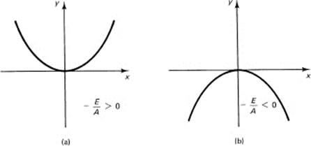
Figure 6.7-1 Parabolas
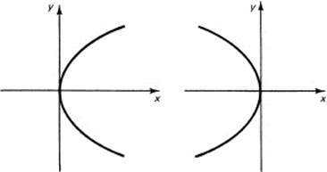
Figure 6.7-2 Parabolas
Example 6.7-1
Given the equation
x2 + 6x – 4y + 1 = 0
you first complete the square on the x term and then adjust the y term properly to get
(x + 3)2 = 4y – 1 + 9 = 4(y + 2)
Translated to the point (–3, –2), you have the parabola
![]()
as shown in Figure 6.7-3.
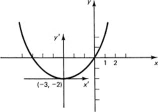
Figure 6.7-3
Example 6.7-2
Given the equation
y2 + x + 4y + 6 = 0
completing the square on the y term gives
(y + 2)2 = – x – 2 = –(x + 2)
Set y + 2 = y′ and x + 2 = x′ to get
(y′)2 = –x′
This clearly requires x′ ≤ 0 and is symmetric with respect to the x-axis (because of the even powers in y). See Figure 6.7-4.
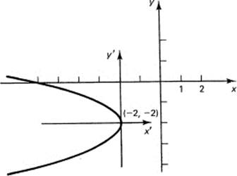
Figure 6.7-4
EXERCISES 6.7
1.Plot x2 = –y.
2.Plot x2 – 6x + y = 7.
3.Plot y2 + 4y – 6x + 3 = 0.
4.Plot y2 – 6y – x = 4.
5.Plot y2 = 2px, with p > 0.Hint: If x = 2p, then y = ± 2p.
6.Plot x2 = 2py, with p < 0.
6.8 MISCELLANEOUS CASES
In our analysis of the general quadratic equation (with the xy term missing), we have now to pick up the missing cases. For example, if both the square terms in the general form (6.4-1) (when reduced by the translation) have negative coefficients, you have
![]()
which is impossible for real numbers; it is an imaginary curve. Indeed, we are apt to say that we have “an imaginary ellipse.”
In the reduction by completing the square when both square terms are present and we find that the right-hand side is zero, then we have either (1) a sum of two squares equal to zero requiring both to be zero, meaning the curve is only one (real) point, or else (2) a difference of two squares, meaning we have a pair of intersecting lines.
Example 6.8-1
These two cases are realized in the following two specific examples.
(1) x2 + y2 = 0
which has only (0, 0) as a (real) solution. And
(2) x2 – y2 = 0
which has solutions
y = ± x
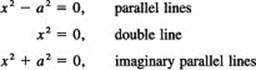
Further degenerate cases can occur, such as
x2 = a2
leading to the two parallel vertical lines
x = a and x = –a
The degenerate case
x2 + a2 = 0
is, of course, a pair of imaginary lines. The case
x2 = 0
is two coincident lines, x = 0 and x = 0. Of course, these degenerate cases can come in many disguises, a simple variation being y in place of x.
EXERCISES 6.8
1.Plot x2 + 4x + y2 = –4.
2.Plot y2 – x2 = 0.
3.Plot x2 = 4.
4.What is the locus of x2 + 1 = 0?
5.What is the locus of y2 = 4?
6.What is the locus of x2 + 4x + 4 = 0?
6.9* ROTATION OF THE COORDINATE AXES
The complete second-degree form
![]()
has, in conventional notation, a cross-product term xy with coefficient 2B. This term may be removed by a rotation of the coordinate axes. Thus we must look briefly at coordinate axes rotations.
We begin with Figure 6.9-1, connecting the old x–y coordinate system with the new x′–y′ coordinate system by a rotation of angle φ (Greek lowercase phi). In the original coordinate system we set
x2 + y2 = r2
![]()
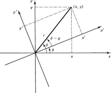
Figure 6.9-1 Rotation
After we rotate an angle ϕ to the new coordinate system, we have the same r, but the angle θ – ϕ as the new angle. Thus we have
x′ = r cos(θ – φ)
y′ = r sin(θ – φ)
We expand the trigonometric functions by the addition formulas (16.1-6) and (16.1-9):
![]()
We note that in the old coordinate system
x = r cos θ
y = r sin θ
and use these to eliminate the occurrences of r in (6.9-3). Hence
![]()
These are the equations of rotation from the old to the new coordinate systems. However, in use it is often the other way around; given the new coordinates x′, y′, we use the above substitutions to get the equation into the old coordinates.
We can find the inverse rotation of (6.9-3) (from the new to the old) by simply multiplying the top equation by cos ϕ and the lower by –sin ϕ to eliminate the y term, and by sin ϕ and cos ϕ, respectively, to eliminate the x term. Using
(cos ϕ)2 + (sin ϕ)2 = 1
we get the transformations
![]()
Observe that (6.9-5) is equivalent to replacing the angle θ by – θ in Equations (6.9-4) for the initial rotation. Thus we know how to transform either way. In particular, given an equation in x, y coordinates, Equations (6.9-5) can be substituted in place of the x and y to get the same geometric features in the new, rotated coordinate system.
It is worth noting that when you want to rotate the axes for an equation you need to have expressions in terms of the old variables, the set (6.9-5); but when you want to transform a point (x, y), you use the other set (6.9-4) and insert the values of the point (x, y) to get the new coordinates (x′, y′) in the primed variables.
We are now ready to show how the xy term can be eliminated by a suitable rotation. Using the transformation (6.9-5) on the general form, we find that only the quadratic terms are involved in determining the actual angle of rotation. We have, after a lot of algebra,
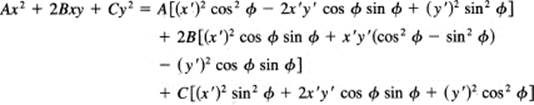
We want to eliminate the x′y′ term, so we must equate its coefficient to zero. Thus we have
![]()
which determines the angle of rotation ϕ. Using the following double-angle formulas (16.1-10) and (16.1-11) (obtained from the addition formulas by setting both angles equal to each other),
![]()
we have
(–A + C) sin 2ϕ + 2B cos 2ϕ = 0
Divide through by (C – A) cos 2ϕ to get
![]()
This determines the particular angle ϕ of rotation that eliminates the xy term. Having eliminated it, we are now ready to proceed as before to determine what geometric curve corresponds to the given equation.
Rotation of the coordinate axes is clearly a messy problem, which we avoid when possible. Therefore, we will illustrate the coordinate rotation with only one example where the amount of the rotation is already given.
Example 6.9-1
Given the special (equilateral) hyperbola (in a sense this corresponds to the circle among the class of all ellipses)
x2 – y2 = 2
we rotate the coordinates by −45°. The rotation (6.9-5) is
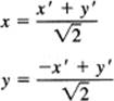
We get
![]()
or, since so many terms cancel,
x′ y′ = 1
Figures 6.9-2a and b show the curves before and after rotation.
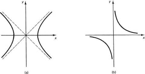
Figure 6.9-2
EXERCISES 6.9
1.Reduce the equation x2 + 2xy + y2 = 1 to standard form.
2.Remove the xy term from xy = 1.
3.Show that B2 – 4AC = (B′)2 – 4A′C′ for any rotation.
6.10* THE GENERAL ANALYSIS
In these days, when the control of a situation is often done in a computing machine, it is necessary to make a complete analysis of all possible situations. In practice, sooner or later, every possible situation that can occur will occur, and if you have not made adequate preparation for it in the computer program, you will almost surely get nonsense out of the computer. However, it will sometimes require an effort on your part to recognize this! Everyone is familiar with the consequences of incompletely analyzed computer programs, so nothing more need be said of the importance of a complete analysis. We will use the quadratic in two variables to illustrate one way of doing such an analysis.
Given the complete quadratic in x and y,
Ax2 + 2Bxy + Cy2 + Dx + Ey + F = 0
if B ≠ 0, then we rotate the coordinate axes (Section 6.9) by the angle ϕ defined by (6.9-6),
![]()
which reduces the quadratic to the form (new letters A, C, D, E, and F in place of the old ones)
Ax2 + Cy2 + Dx + Ey + F = 0
If A = C, then ϕ = 45°. We now have B = 0.
We continue with the analysis. At this point there are three cases to be examined, depending on the presence of the square terms.
Case I
Both terms present (AC ≠ 0) (Section 6.3). You get after completing the square
![]()
where
![]()
We now have two subcases depending on whether K is or is not 0. If K ≠ 0, then we can divide through by it and write the equation in the form
![]()
There are three possibilities, depending on the ± signs.
1.Both plus: ellipse (Section 6.5)
2.Opposite signs: hyperbola (Section 6.6)
3.Both negative: imaginary curve (Section 6.8)
If K = 0, then we have the degenerate case of Section 6.8. If both the signs are the same, then it is imaginary, and if they are different then you can factor it into two intersecting lines (Section 6.8).
Case II
One square term only. We have parabolas (Section 6.7) provided both variables x and y are present. If only one variable is present, there are three possible cases having the typical forms:
These equations could be in the variable y instead, and remember we are talking about the situation after a rotation to remove any xy term that may be present.
Case III
No square terms. This means that if we translated and rotated back to the original equation we would still have a linear equation, a straight line. Therefore, the original given quadratic was in fact linear in x and y, that there were no original quadratic terms, that A = B = C = 0. We must allow, of course, for further degenerate cases including all the coefficients equal to zero.
We now examine our analysis and arrange it in a logical form.
1.If B ≠ 0, then you rotate the coordinate system to make the cross-product term vanish. Thus you are reduced to the case of B = 0 from now on.
2.If AC ≠ 0 (both square terms are present), you complete the squares in both variables. There are two cases to consider depending on the K term. If K ≠ 0, then we have (a) the ellipse when both coefficients are positive, (b) the imaginary ellipse when both terms are negative, and (c) the hyperbola when the two terms have opposite signs. If K = 0, then if the signs are different the equation factors into two lines (the asymptotes of the hyperbola when the K ≠ 0); while if the signs are the same, then it is a pair of imaginary lines.
3.If AC = 0, then one square term is missing, and you have a parabola when the other variable is still present, and a square of the variable if the other is missing. This square leads to (a) parallel real lines, (b) imaginary parallel lines, or (c) coincident lines depending on the value of the constant term.
4.If both A = 0 and C = 0 (after the possible rotation), then you did not have a quadratic to begin with.
6.11 SYMMETRY
Symmetry is a fundamental concept in mathematics. At the moment, we are concerned with geometric symmetry. Symmetry of two points with respect to a given line L requires that the line segment joining the two points be bisected perpendicularly by the given line L (Figure 6.11-1). In mathematics, given the points (x1, y1) and (x2, y2), the midpoint of the line segment (see example 5.6-3) is clearly
![]()
This point must lie on the line L of symmetry, and the two, lines must be perpendicular.
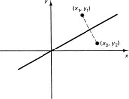
Figure 6.11-1 Line of symmetry passes through origin
The special cases of symmetry with respect to the x-axis require that the y coordinates of symmetric points be equal in size and opposite in sign. If the function depends only on y2, then both y and –y will (or will not) satisfy the equation (Figure 6.11-2).
Similarly, symmetry with respect to the y-axis requires the formula to have only even powers in x (although, of course, there can be y terms and constant terms) (Figure 6.11-3).
The reduced ellipses and hyperbolas (6.4-4) have both x- and y-axis symmetries. The parabola when reduced has only one of these symmetries.
Next in importance is the case of symmetry with respect to the 45° line. For this case the symmetric points are (x, y) and (y, x); you simply interchange the x and y
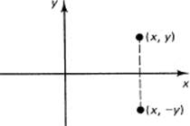
Figure 6.11-2 Symmetry with respect to the x-axis
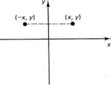
Figure 6.11-3 Symmetry with respect to the y-axis
coordinates! This is easily seen from Figure 6.11-4. For example, the equation (a quartic)
x2y2 = 1
has all three types of symmetry. The rotated hyperbola xy = 1 has symmetry with respect to the 45° line.
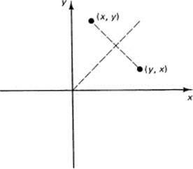
Figure 6.11-4 Symmetry with respect to the 45° line
Symmetry with respect to the 45° line is easily described by the words, “They are inverse functions of each other.” Thus the parabolas
x = y2 and y = x2
are inverse functions (see Figure 6.11-5). One branch of x = y2 is
y = ![]()
and the other branch has the minus sign.
There is also symmetry with respect to a point, typically with respect to the origin. Here if we have the point (x, y), we must also have the corresponding point (–x, –y) (Figure 6.11-6). The ellipses and hyperbolas when reduced have this symmetry. Indeed, if a curve has two of the three symmetries, x-axis, y-axis, and origin symmetry, then it has the third.
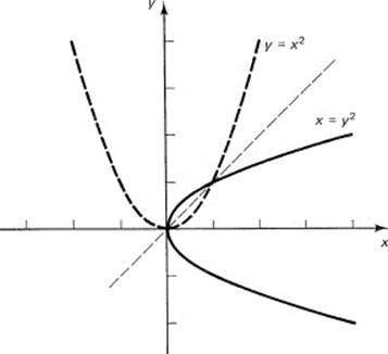
Figure 6.11-5 Inverse functions
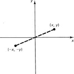
Figure 6.11-6 Symmetry with respect to the origin
There is also rotational symmetry. A circle has perfect rotational symmetry; any rotation must leave the equation unaltered. A square centered about the origin has rotational symmetry of ±90°, ±180°, ±270°, …. Similarly, for any regular polygon about the origin, there are the corresponding symmetries.
How can one remember all these rules? You do not even try! All symmetries come from the invariance of the equation under the appropriate change of variables. Fundamentally, you look for changes of variables that will leave the equation invariant. That is all there is to geometric symmetry! Common invariances are x → –x, y → –y, separately or together, and interchange of x and y. You have only to learn to think, “What point goes into what point?” to grasp the corresponding symmetry.
EXERCISES 6.11
1.*Show that a circle centered about the origin has rotational symmetry by making an arbitrary rotation of its equation.
2.Prove by algebra that if two of the symmetries mentioned above occur then the third must occur.
3.Discuss the symmetry for the equation x2 = f(y). For y2 = g(x).
4.What symmetry has the equation f(x, y) = f(y, x)?
5.What symmetry has the equation f(x, y) = f(–x, –y)?
6.12 NONGEOMETRIC GRAPHING
The discussion has been, so far, about geometric figures. In geometry we believe that the plane is isotropic, the same in every direction. But in practice we often plot nongeometric relationships in rectangular coordinates, say dollars versus years. There is no common measure of such different quantities as dollars and years; either axis can have its units chosen independently of the other. Thus there is no meaning to rotation in such a coordinate system since the rotation formulas would have you adding dollars to years (apples to oranges in the classical example in beginning algebra).
Similarly, there is no meaning to the slope of a line. Instead, we fall back on the rate of change, a change of so many dollars per year. The slope itself has no meaning except in two cases, zero slope and vertical slope. In such cases the change of the unit size in one variable does not affect the tilt of those lines. Scale transformations
![]()
are a special case of affine transformations, and therefore scaling geometry (6.12-1) is a special case of affine geometry.
Thus we need to be wary about when we use rotations; they are appropriate only when the coordinate axes have the same units.
6.13 SUMMARY OF ANALYTIC GEOMETRY
The basis for analytic geometry is that a pair of numbers corresponds to a unique point in a plane, and conversely. Similarly, equations and curves correspond (almost). In particular, straight lines correspond to linear equations, while quadratic equations correspond to the conics (the ellipses, hyperbolas, parabolas, and degenerate pairs of straight lines). These conics occur in many places: a single small planet about a massive sun moves in an ellipse, as does a satellite about the earth (neglecting perturbing effects of other planets and the sun, and assuming Newtonian mechanics, but not relativity); higher-speed particles from outer space may move in a hyperbolic orbit (similarly a satellite may acquire sufficient energy and then move in a hyperbolic orbit); and telescope mirrors (as well as automobile headlights) have a parabolic shape.
It is necessary to point out that, although you tend to equate in your mind “function” and “graph,” there are significant differences. A function, by definition, must be single valued, while many equations have multiple values (for example, a circle).
You should learn to go from the geometric properties to the algebraic properties and back for each kind of object and equation. We have glossed over many of the details and barely discussed the rotation of coordinates because they are not of great interest in this course, although they can be in some situations. We have also ignored many details of the conics, which may be found in texts specially devoted to them.