Methods of Mathematics Applied to Calculus, Probability, and Statistics (1985)
Part II. THE CALCULUS OF ALGEBRAIC FUNCTIONS
Chapter 8. Geometric Applications
8.1 TANGENT AND NORMAL LINES
To a great extent, the differential calculus arose from the problem of finding the tangent line to a given curve at an arbitrary point. We have just seen how to find the slope of a curve at an arbitrary point (x, y); it is simply the derivative of the function at that point.
To find the tangent line, we could assume the general form of a straight line (Section 5.4)
![]()
and impose the two conditions (using the method of undetermined coefficients) that the line pass through the point and have the given slope at that point. The resulting two equations would be linear (in the unknown coefficients) and easy to solve (there really are only two parameters in the general form of the equation). Because we now want to use the symbols x and y for points running along the tangent line, it is necessary to fix the point where the line is to be tangent; call the point on the curve (x1, y1). This is the point where we impose both the point and slope conditions. As an alternative to (8.1-1), we can use the more convenient point-slope form of the line, Equation (5.6-6):
![]()
where, of course, m is the slope (the derivative of the curve at the point (x1, y1)).
Example 8.1-1
Suppose we use the simple parabola as a test case,
y = x2
The derivative at the point (x1, y1) is
![]()
Therefore, the tangent line at the point (x1, y1) is
y − y1 = 2x1(x − x1)
In particular, at the point (1, 1) on the curve, we have
y − 1 = 2(x − 1)
ory = 2x − 1
See Figure 8.1-1.
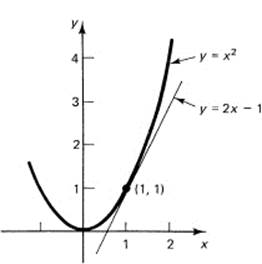
Figure 8.1-1 Tangent to a parabola
Besides asking what is the tangent line at a given point, we can ask many other questions such as: “Where does a given curve have a slope parallel to a given line?”
Example 8.1-2
Where does the parabola
y = x2
have a tangent parallel to the line
y = 3x
(Figure 8.1-2)? The word “parallel” means “having the same slope.” The slope of the given line is 3 (either from the point-slope formula or by differentiating the equation for the line). We equate this to the slope of the parabola (2x)
2x = 3
which tells us that, at the place where ![]() and (from the equation of the parabola)
and (from the equation of the parabola) ![]() the tangent to the parabola is parallel to the given line. The actual tangent line is
the tangent to the parabola is parallel to the given line. The actual tangent line is
![]()
or ![]()
We can check this easily. Is the slope right? Does it pass through the required point? Both the original line and the solution line have the same slope 3. Thus it remains to check that the point ![]() lies on both the parabola (obviously) and on the solution line. We have, putting the coordinates of the point into the equation of the line,
lies on both the parabola (obviously) and on the solution line. We have, putting the coordinates of the point into the equation of the line,
![]()
as it should.
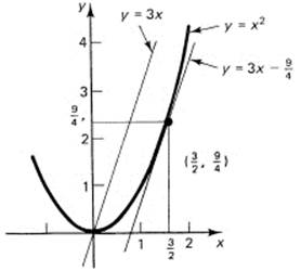
Figure 8.1-2 Parallel tangent line
Example 8.1-3
We may also ask where two curves are tangent to each other. For example, which parabola of the family (depending on the choice of a)
y = ax2
is tangent to the line
y = x + 1
and at what point?
We require two conditions: (1) the two curves meet at a point, and (2) the two curves have the same slope at that point. In mathematical terms, we require both
(1) 2ax2 = x + 1
and
(2) 2ax = 1
To eliminate the a, multiply the first equation by 2 and the second equation by –x and add. You get
0 = 2x + 2 − x
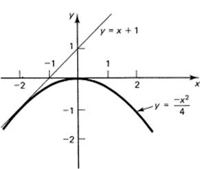
Figure 8.1-3 Parabola tangent to a line
which yields x = –2, y = –1 (from the line), and hence ![]() (from the parabola).
(from the parabola).
This is easily checked by sketching the two curves (Figure 8.1-3).
The normal line is the line perpendicular to the tangent line that passes through the point of tangency. We recall from Equation (5.5-8) that two lines are perpendicular to each other when their slopes are the negative reciprocals of each other. Thus, to find the normal line, we use the negative reciprocal of the derivative as the slope; otherwise, things are the same.
Example 8.1-4
Using the same parabola,
y = x2
and the same point, (1, 1), find the normal line. The slope of the curve at the point is m = 2. The negative reciprocal is ![]() Thus the normal line is
Thus the normal line is
![]()
or
![]()
See Figure 8.1-4. Again, it is easy to check the answer.
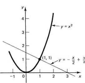
Figure 8.1-4 Normal line
EXERCISES 8.1
Find the tangent and normal lines to the curve at the indicated point:
1.y = x3 at (1, 1)
2.y = x4 at (1,1)
3.y =1/x at (1,1)
4.y = x + 1 at (0,1)
5.![]() at (1,1)
at (1,1)
6.![]() at (1, 1)
at (1, 1)
7.y = xn at (1, 1)
8.y = ax2 + bx + c at (x1, y1)
9.Show that the normal line to the semicircle ![]() passes through the center of the circle.
passes through the center of the circle.
8.2 HIGHER DERIVATIVES—NOTATION
From a given function
y = y(x)
we derived a function, called the derivative,
![]()
This is a function of x, and therefore we can again apply the process of differentiation; we can compute
![]()
Example 8.2-1
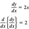
For the usual parabola
y = x2
we have the first and second derivatives
For the more complicated function (the upper branch of a circle)
![]()
we have
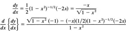
or
![]()
This notation for the second derivative is clearly a nuisance. Traditionally (using the observations of Section 2.8 on the use of exponents on symbols), it follows that
![]()
is the second derivative. The third derivative would be
![]()
and, in general, the nth derivative would be
![]()
Remember that d/dx is a single symbol. Nevertheless, conventionally it is written as
![]()
the last being clearly a convenience. Read this as a single symbol, “d to the nth over dx to the nth”.
The derivative is often written in shorter forms. For example, all the following notations are in widespread use
![]()
The use of the prime notation (y prime) is especially convenient. The higher derivatives are correspondingly
![]()
and so on. We will often use the prime notation (y″, pronounced “y double prime,” for example).
EXERCISES 8.2
Find the first and second derivatives of the following:
1.![]()
2.y = xn
3.![]()
4.y = 1/x
Find the third derivative of the following:
5.y = x3, xn, 1/x, ![]()
6.Show that the nth derivative of a polynomial of degree n is ann!, and that the (n + 1)st derivative is zero.
Find the nth derivative of the following:
7.y = 1/x
8.y = ![]()
9.y = (a + bx)m
8.3 IMPLICIT DIFFERENTIATION
Example 8.3-1
The conventional form of a circle
x2 + y2 = r2
requires us (at present) to solve for one branch or the other,
![]()
depending on which piece of the double-valued function we want to use. However, we can avoid the unpleasantness of the square roots during the differentiation process by a process called implicit differentiation. Take the equation of the circle in the conventional form,
x2 + y2 = r2
and start the four-step delta process (Section 7.5). We will get, at step 2 of the four-step process,
![]()
Now subtract the original equation and divide by Δx. We get
![]()
We then take the limit as Δx approaches 0, noting that as Δx → 0 it also follows that Δy → 0. We get
![]()
This shows that we simply apply the rule for “differentiating a function of a function” to the y terms. The final result in the case of a circle is
![]()
The value of y we use selects the branch we are on.
Example 8.3-2
Suppose we have the hyperbola
xy = a2
Differentiate the product to get
![]()
or
![]()
Example 8.3-3
Find the angle of intersection between the circle x2 + y2 = 5 and the hyperbola xy = 2 in the first quadrant.
You must first find the point of intersection. To find it you (cleverly) add and subtract twice the hyperbola equation from the circle equation to get
x2 + 2xy + y2 = 5 + 4 = 9
x2 – 2xy + y2 = 5 – 4 = 1
Take the square root of both equations, from which the solutions are
x + y = ±3
x − y = ±1
Remember that the solution is to be in the first quadrant. You get, after some thinking and the use of symmetry,
x = 2, y = 1 and x = 1, y = 2
Check that that both points lie on both curves! From Example 8.3-1 for the circle at the point (2, 1),
![]()
and for the hyperbola, Example 8.3-2,
![]()
We now look back, Equation (5.5-5), for the formula for the angle between the two tangent lines. At the point of intersection we have
![]()
from which (see Figure 8.3-1) θ is approximately –37°. From symmetry, the size of the angle at the second point is the same, although the sign will be different.
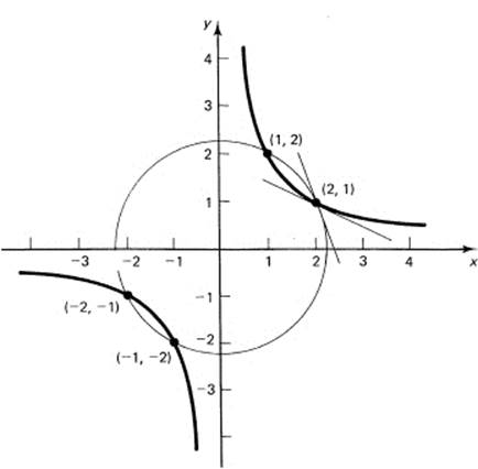
Figure 8.3-1 Angle between a circle and a hyperbola
Example 8.3-4
Suppose we have the more complex expression
x2y2 + 5y − x4 − 5 = 0
To find the slope at any point, we simply differentiate according to the usual rules. The first terms is a product. We have
![]()
and solve for dy/dx:
![]()
or
![]()
At the particular point (1,1), which lies on the original curve, the slope is
![]()
We could, of course, also compute the second derivative if we wished.
Notice how implicit differentiation lures us out of the domain where y is a single-valued function of x. Implicit differentiation is a very useful tool in many situations where we are initially given implicitly defined functions, rather than the conventional explicitly defined, single-valued function.
EXERCISES 8.3
Find dy/dx for the following:
1.x2/a2 + y2/b2 = 1 at the point (a/![]() , b/
, b/![]() )
)
2.x3y3 = 1 at the point (1, 1)
3.x3 + y3 = 2a3 at the point (a, a)
4.x2 + 3xy + y2 = 5a2 at the point (a, a)
5.![]() at the point (1,1)
at the point (1,1)
6.(x2 – y2)/(x2 + y2) = 1 at the point (1, 0)
Find the tangent and normal lines to the following:
7.x3 + y3 = 2a3 at (a, a)
8.1/x + 1/y = 2 at (1, 1)
9.x2/a2 + y2/b2 = 1 at (a/![]() , b/
, b/![]() )
)
10.Generalize Exercise 7. Describe the result geometrically and algebraically.
8.4 CURVATURE
If we can fit a straight line (having two parameters) to a curve at a point using the two conditions of matching both point and slope at the point, then clearly we can extend the idea and fit a circle, which has three parameters, by matching at a point on the curve the three conditions of point, slope, and second derivative. By fitting a circle, we can measure the curvature of the function at a point. This gives us some additional information about the function.
To fit the circle, we could use the general form (6.2-3) of the circle (with D, E, and F as linear undetermined parameters); but since it is likely that we will want the geometrical properties of the circle (the center and radius), it seems better to pick the form (6.2-1):
![]()
In this form the unknown parameters h, k, and r occur nonlinearly, but since we believe we could solve the linear form using D, E, and F as the variables and then reduce it to the present form, probably we can handle this nonlinear case of undetermined coefficients (if we are careful!). After all, the solution must be the same either way we solve it.
Implicit differentiation of (8.4-1) gives
![]()
Differentiating again, we get
![]()
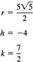
The unknowns are the values of h, k, and r. The knowns are the point (x, y), slope y′, and second derivative y″. Equation (8.4-3) can be solved for
![]()
Equation (8.4-2) can be solved for
![]()
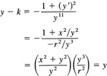
These two equations give the coordinates of the center (h, k) of the circle. Put (8.4-5) in the first Equation (8.4-1) to eliminate the parameter h:
![]()
Now eliminating the (y – k) from (8.4-6) and (8.4-4), we have the radius
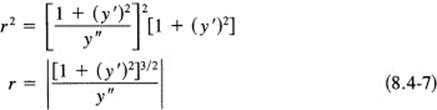
The absolute value occurs because by convention the radius of a circle is a positive quantity.
This is the radius of the circle that fits locally the curve (matches point, slope, and second derivative). Hence r is called the radius of curvature. This circle is sometimes called the osculating circle (osculate means to kiss).
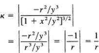
If the original curve had been a straight line, or if the particular point of the curve we were using had the second derivative equal to 0, then we could not divide by it to get the radius of curvature. We say, glibly, “The radius of curvature is infinite.” Because of this possibility, we often prefer to talk about the reciprocal of the radius of curvature, and call it the curvature,
![]()
(κ is Greek lowercase kappa). Thus a straight line has zero curvature.
Example 8.4-1
For the circle
x2 + y2 = r2
we know the center is (0, 0) and the radius is r. This makes a good test of the above formulas and of their derivation. First, differentiate implicitly to get
![]()
Divide out the factor 2, and solve for y:
![]()
Differentiate this again:
![]()
Eliminate the y′ to get
![]()
We have therefore (8.4-8)
which is independent of x and y, as it should be for a circle. To find the center of this circle, we use formulas (8.4-4) and (8.4-5). First we find k from the Equation (8.4-4):
Therefore, k = 0. Similarly, we find h from (8.4-5):
![]()
And h = 0 as it should. The formulas pass this obvious test.
Example 8.4-2
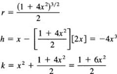
Suppose we find the radius and center of curvature for the parabola (Figure 8.4-1)
![]()
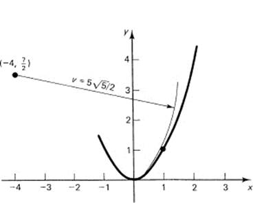
Figure 8.4-1 Osculating circles
Therefore, from (8.4-7), (8.4-5), and (8.4-4),
We can check this easily at the point (0, 0). We have r = ![]() , h = 0, and k =
, h = 0, and k = ![]() . As another check, we can try the point (1, 1). Again, see Figure 8.4-1. We get
. As another check, we can try the point (1, 1). Again, see Figure 8.4-1. We get
The distance from (h, k) to the point (1, 1) must be the radius of the circle. Hence
![]()
Again, things check properly.
Generalization 8.4-3
Suppose we try to extend the above sequence of matching (1) the point, (2) the tangent line, and (3) the second derivative to find the matching circle. What curve would be sensible to fit to the function, first, second, and third derivatives? The next convenient geometric figure we know much about is the general ellipse (or hyperbola), which has six parameters. If we used this, we would have to go up to fitting the fifth derivative. We can certainly do this, because the parameters enter in linearly and the corresponding linear equations will be solvable in general (although degenerate cases of local straight lines and the like could arise). But we would not know how to interpret the result if we got it! The generalization is probably not worth the effort.
We see how we can fit locally curves from one given family of curves to another given curve at a given point; we see the essence of local approximation methods. “Local approximation” means “fit as many consecutive derivatives (the function is the zeroth derivative) as you can.” If you try skipping some of the derivatives, you can get into trouble.
EXERCISES 8.4
1.Find the center and radius of curvature for the function y = xn at the point (0, 0), and check by using n = 2.
2.Find the curvature of the function y = 1/(1 + x2) at x = 0.
3.Find the curvature of y2 = a2 + x2 at (0, a)
4.Find the curvature of x2/3 + y2/3 = a2/3 at (a, 0).
5.Find the curvature of y = a1/3x2/3 at (a, a).
8.5 MAXIMA AND MINIMA
At a local maximum or minimum of a curve where the function has a derivative (see Figure 8.5-1), the slope must be 0. We use this observation backward when we are asked to find the local maximum or minimum of a curve (the best or worst). Simply set the derivative equal to 0 and find where this can happen (i.e., where the tangent is horizontal). It may be, as at point C in the figure, that the slope is horizontal, and that it is neither a local maximum nor a local minimum.
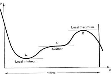
Figure 8.5-1 Local maxima and minima
Furthermore, if you are to find the maximum or minimum in an interval, say – 1 ≤ x ≤ 1, it may happen that the extreme value occurs at one end of the interval, and the slope of the tangent line is not necessarily 0.
Example 8.5-1
As a simple example, consider maximizing the area of a rectangle with a given fixed perimeter. In word problems like this, you pick symbols for the quantities and write down the statements (see Figure 8.5-2). Let the rectangle have dimensions x and y. The total perimeter, P, of the rectangle is
P = 2x + 2y
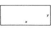
Figure 8.5-2 Rectangle
This is a condition between x and y. (Of course, we limit x and y to be nonnegative.)
The area, A, which is what we want to maximize, is
A = xy
It is easy to eliminate one of the variables using the side condition (the perimeter P is fixed). Thus, to eliminate y, we have from the perimeter equation
![]()
Put this in the area expression to get
![]()
We see, after a moment, that this is a parabola opening downward (consider large positive and negative x and see what happens), so there is a maximum somewhere.
The slope of the curve (= slope of the tangent line) of A = A(x) is given by
![]()
At the maximum, this derivative must be zero, so we have

Using the perimeter equation for y, it follows that
![]()
so we have a square as expected.
It is important in learning to do mathematics to review what is done and why it was successful. The common remark that you should learn from your mistakes is misleading; there are so many ways of being wrong and so few ways of being right that it is usually better to study successes.
What did we do? First, we took the statement of the problem and converted it to symbols and then to equations. Never underestimate the power that simply naming things gives you. Next, we eliminated all but one of the variables; in this case we eliminated y. Then to find the maximum, which we had convinced ourselves was there, we differentiated and set the derivative equal to zero. We solved this equation and substituted back into the earlier relationships to get the unknowns x and y. Then we interpreted the results; x = y means that we have a square. Notice that we chose a form for stating the answer that eliminates reference to both P and A; we described the nature of the solution, not the specific details.
It is worth noting that among rectangles the shape, a square, is the solution for the equivalent problem; for a fixed area, find the shape with the minimum perimeter. Why are the two problems equivalent?
Example 8.5-2
A very similar problem is that of building a rectangular-shaped fence along a river or the side of a sufficiently long bam (which saves one side of the fencing). The amount of fence is fixed, and you want the maximum amount of enclosed rectangular area. Again, we pick the variables xand y for the dimensions, y in the direction of the river or bam, and x perpendicular to y (see Figure 8.5-3). The perimeter this time is
P = 2x + y
and the area again is
A = xy
Again, eliminate the variable y; this time
y = P – 2x
and the area is
A = x(P – 2x) = Px – 2x2
This is a parabola opening downward, so there is one maximum. To find the maximum, differentiate and equate to 0.
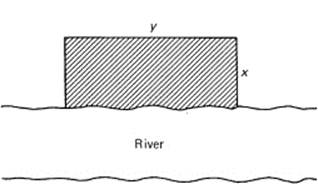
Figure 8.5-3 Minimum perimeter
![]()
or
![]()
Therefore,
![]()
The “shape” of the field is, say, the ratio of x to y:
![]()
This expresses the answer in a form that is independent of the particular given length of fence.
Example 8.5-3
You are given a square sheet of paper or metal, and wish to cut out square comers and then fold up the sides to make a shallow tray. Find the shape of the tray with maximum volume.
Let the given square have sides of length L (if you must be specific think of L = 17), and let x be the side of the small comer squares you are going to cut out (see Figure 8.5-4). The volume is then (height times the square base)
![]()
Therefore,
![]()
gives the maximum. Factor this:
(L − 2x)(L − 6x) = 0
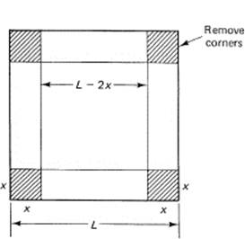
Figure 8.5-4 Shallow tray
The solution L = 2x is clearly zero volume (minimum volume); it is the other solution
![]()
that you want. The bottom dimension is therefore
![]()
So the shape, the depth to width, is
![]()
Word problems are the bane of many a student’s existence. One of the simplest errors is that when finally the x value of the extreme is found the student forgets that this is but a step toward the final answer, and fails to find what was asked for. There are no simple rules for solving word problems in a mechanical fashion. Indeed, in doing research it is the ability to go from vaguely formulated problems to the “proper” clear formulation that marks the great scientist from the average person. Einstein repeatedly said that he “had a nose” for smelling out the right approaches, and an examination of biographies of his life indicates the truth of this observation. The great people differ from the run-of-the-mill able people by their ability to formulate questions “properly.” Thus, if you want to use the mathematics you are learning, you need to pay attention to this aspect of the course. The formulation of a real problem requires a good deal of idealization of reality; just which idealization you choose measures, in some sense, your ability to do things “right.” It is the ability to select the relevant and ignore the irrelevant aspects of a problem that matters.
Example 8.5-4
What is the optimal shape of a closed cylinder? What do we mean by optimal? What can it mean? It could mean, for example, that for a given volume the surface is minimal. Or it could mean that for a fixed surface the volume is maximal. Some thought shows that in this case the two are the same question! See Figure 8.5-5.
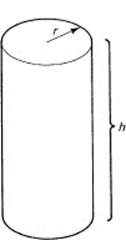
Figure 8.5-5 Optimal cylinder
Next, you need some technical knowledge, such as the area of the surface of a cylinder and its volume. The need for technical knowledge is common to all applications: you must know the technical details of the domain of application. The method of finding the optimum, however, is the same. First, introduce some notation. For the cylinder let the radius of the base be r and the height be h. Next, set up the equation for the side area of the cylinder, which is the circumference of the base times the altitude (imagine a can cut up the side and laid out flat). Therefore, the area of the side is
(2πr)h
To this you must add the area of the two ends:
2(πr2)
Thus, the total surface area S is the sum of the two terms:
S = 2πr(h + r)
On the other hand, the volume V is the area of the base times the altitude,
V = πr2h
The third step is to reorganize the equations for your convenience. Suppose you decide to maximize the volume subject to a fixed area. You can eliminate h using the fixed amount of surface equation to find h. This gives
![]()
Therefore, the volume can be written, after a little algebra, as
![]()
This is the volume you want to maximize.
The fourth step is to differentiate with respect to the variable, which in this case is the radius r, and set the derivative equal to 0. You get
![]()
Therefore, solving for the radius r you have
![]()
Next, you need to find h (which is given by the equation used to eliminate it) in terms of r. Substitute the value of r into the equation you used to eliminate h:
![]()
After some algebra you will get
![]()
Is this the answer? No. Look at the question, “What is the optimal shape …?” The shape must mean the ratio of the two sizes. You can take either height to diameter, D, or diameter to height. In the first case
![]()
It is clearly better to state it in terms of diameter than it is to state the result in terms of the radius. The statement height = diameter is the kind of thing you can remember and visualize; when you use the radius, you get an extra factor of 2. Often the value of a result lies in the neat statement of it, so to be an effective person you need to learn the gentle art of presenting the results in a suitable form.
As we earlier observed, in a textbook it is necessary to give very simple examples, but in practice often a single problem may require hours, days, or weeks of work. There is not time in a course to give such problems, but we can give one slightly harder problem and discuss some of the things that arise.
Case Study 8.5-5
Suppose, as in the shallow tray problem, we are again given a square, but this time are asked to form a square pyramid (including the base). We first sketch Figure 8.5-6. Before taking action, we do a little thinking. The result is that maybe Figure 8.5-7 would be a better plan. Are we sure? Well, if we had the optimal solution in the first case, we could rotate it and then have room to make the sides of the pyramid longer. Or could we rotate? Might not the comers of the base hit the sides? Well, a moment’s inspection shows that the base cannot be bigger than half the original side since the flaps must at least meet at the center when folded up. Yes, we could rotate, and we need examine only the second case.
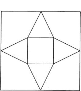
Figure 8.5-6
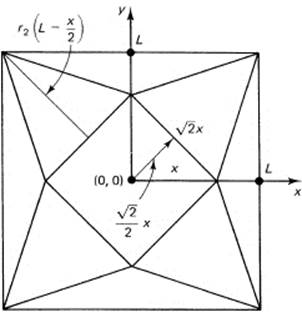
Figure 8.5-7
Due to the symmetry of the figure, it is probably best to pick the origin of the coordinate system at the center. (Rule: Try to use any symmetry you have.) We therefore pick the side of the square to be 2L. Let x be the distance out from the center to the comer of the base. The side of the base is, by the distance formula,
![]()
Therefore, the distance from the origin to the side is one-half of this:
![]()
The distance from the origin to the comer of the square is
![]()
so the slant height of the face to be folded up is
![]()
Now, looking at Figure 8.5-8, the altitude is
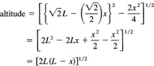
Finally, the volume of a pyramid is one-third of the volume of the corresponding rectangular cylinder; that is
When we differentiate the volume with respect to the variable x and set it equal to 0, the front constant can then be divided out, so we can ignore it. The derivative of the rest, which is a product form, is
![]()
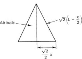
Figure 8.5-8 Altitude of a pyramid
Multiply through by the denominator to get
-x2 + 4x(L − x) = x
or
4x(L − x) = x2
One solution is x = 0, which is of course a minimum. The other solution is
4L − 4x = x
or
![]()
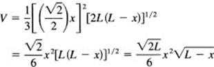
What is the altitude? We look back for the expression for it:
![]()
from which we can find the volume easily. The shape factor would be, probably, the ratio of the altitude to the side of the base,
![]()
The corresponding volume is
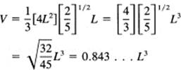
The experienced person would recognize that the answer would turn out to be linear in L for the altitude, and the volume would be proportional to the cube of L. Thus in place of the choice we made for x you could choose xL; the fraction of the edge length could be chosen as the unknown. We have ignored the question of a clever cutting up of the square and later fastening together the parts; we have used the cut and fold condition.
Example 8.5-6
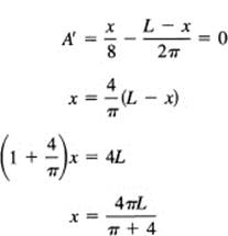
A wire of length L is to be cut into two pieces. The first is formed into a square and the second into a circle. Find where to cut the wire to get the maximum enclosed area. Let
![]()
The area of the square is (x/4)2. The radius of the circle is (L – x)/2π. Hence the area of the circle is π[(L – x)/2π]2. Therefore, the total area is
![]()
We differentiate and set equal to zero.
But when you compute this you find that it is a minimum and that the maximum occurs for x = 0, at one end of the range. Once you realize this, then looking at the original function A you see that it is a parabola opening upward, and that the horizontal derivative must give the minimum, not the maximum. It is then a matter of deciding which end is the larger. The front coefficients on the two terms tells you which is best.
Aside 8.5-7
It may come as a surprise to you to realize that some reasonable sounding problems do not have, for example, a minimum. Consider Figure 8.5-9, two towns A and B, with B due east of A. You are required to depart from A in a northerly direction. Clearly, there is no shortest path that satisfies all the conditions. Only “well-formulated problems” have a unique solution (whatever well formulated may mean in general). This means that in some cases you have to decide if the problem posed to you makes sense or not.
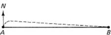
Figure 8.5-9 Shortest path does not exist
EXERCISES 8.5
See Appendix B for the common formulas from geometry.
1.Find the shape of the isoceles triangle along a river having maximum area for fixed length of the two equal legs.
2.Compare the solution of the cylindrical can problem with those in the stores. Why are there differences? What kinds of things did we neglect?
3.Find the depth of the shallow tray of maximum volume made from a piece of material with sides a and b in dimensions.
4.Optimize a tin can with no top. Compare this to the one with a top.
5.Find the maximum volume of a cone that can be put in a sphere of radius a.
6.Find the maximum volume of a right cylinder that can be put in a cone of radius R and height H.
7.A rectangle is surmounted by an equilateral triangle. Find the maximum area for a fixed exterior perimeter.
8.Find the maximum rectangle you can put in an ellipse.
9.Two spheres of radius respectively a and b have their centers c units apart (c > a + b). Find the point where the combined maximum surface can be seen, given that the surface area that can be seen is A = 2πrh, where h is the depth of the sector.
10.Find the largest right circular cylinder that can be put in a sphere of radius a.
11.The heat from a source varies inversely with the distance away. Given two sources of intensities a and b separated by a distance c, find the point between the sources where the intensity is least.
12.Find the largest rectangle that can be put inside the common area of two parabolas, 3y = 12 – x2 and 6y = x2 – 12.
13.A right circular cylinder is topped with a hemisphere (but no bottom). Find the shape for a fixed total surface that has maximum volume.
14.A window is surmounted by a semicircle. Find dimensions for the fixed perimeter that admits the most light.
15.A strip of metal is to be shaped into the cross section of an isoceles triangle with height y and width x. Find the shape with maximum cross-sectional area.
16.Generalize Example 8.5-6. The interesting point about this example is that the maximum occurs at the end of the interval. We therefore ask: (a) Does it depend on using a circle and a square? (b) Would any two regular figures do? (c) Would any two systems of similar convex figures do? (d) Must they be convex? (e) Could the edges of a figure shape cross itself? (f) What determines which end will have the extreme?
8.6 INFLECTION POINTS
In Section 8.4 we found the circle that best fitted a given curve at a point. As the point where we fit the local circle to a curve moves along the curve, we find that the curvature is continually changing. This osculating circle and its curvature are properties of the curve, since they do not change when the coordinate system is shifted or rotated. The curvature is an intrinsic property of the curve.
We now introduce a similar concept, but one that is tied to the coordinate system. This idea uses the words “concave” and “convex.” Consider the simple curve
y = x3
(see Figure 8.6-1). On the right side the curve is concave up (convex down), and on the left it is concave down (convex up). Between them there is a point where it is neither, the origin. Such a point, where the curve changes from concave up to concave down, we call an inflection point. Where the curve is concave up, the second derivative is positive, and where the curve is concave down, the second derivative is negative. Where it is neither concave up nor concave down, the second derivative is zero. Such a point is called an inflection point. That the condition y′ = 0 is not always an inflection point follows from an examination of the simple curve
y = x4
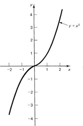
Figure 8.6-1 Inflection point
The second derivative is (see Figure 8.6-2)
y′ = 12x2
and at the orgin this is zero, although there is no change in the convexity upward. Thus the vanishing of the second derivative is a necessary but not sufficient condition for an inflection point. At an inflection point the tangent line crosses the curve.
To get a feeling for the matter in the general case, we start with a sketch of some curve (see the top of Figure 8.6-3). Below this curve we sketch the curve of its derivative, using the simple fact that positive slopes must have derivative values that are positive and negative slopes have negative derivative values. See again Figure 8.6-3. If we now repeat the process of sketching the derived curve from a given curve,
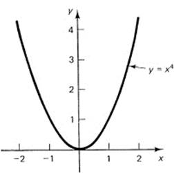
Figure 8.6-2 No inflection point
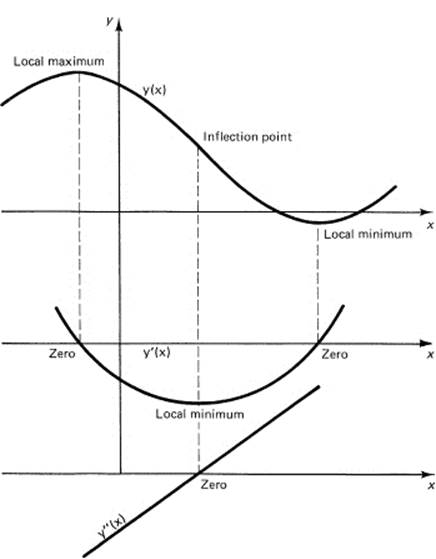
Figure 8.6-3
we are led to the second derivative curve shown at the bottom of the figure. Where the second derivative crosses the x-axis, the top curve has a change in curvature.
Example 8.6-1
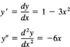
Consider the simple cubic (Figure 8.6-4)
y = x(1 – x2) = x – x3
The first two derivatives are
Equating the first derivative to 0 gives the positions of the local maxima and minima:
![]()
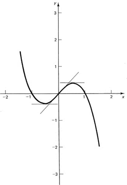
Figure 8.6-4 A cubic
Equating the second derivative to 0 gives the position of any possible inflection point:
x = 0
We need the corresponding function values at these points. For the max-min points
![]()
For the inflection point at x = 0, evidently y = 0. It is now easy to sketch the curve. The only additional information we might need would be the slope at the inflection point, which is exactly 1.
If we examine the idea of a local minimum closely, we see that as we go from left to right the slope passes from negative values to positive values, and this means that the second derivative must be positive. On the other hand, at a local maximum the slope passes from positive to negative, and the second derivative must be negative. Thus we have the following rule:
At a local minimum the second derivative is ≥ 0. At a local maximum the second derivative is ≤ 0.
The rule can best be remembered by Figure 8.6-5 and the soup bowls. A bowl will hold the soup, be +, when it is concave up and will not hold the soup, be −, when it is concave down.
![]()
Figure 8.6-5 Soup bowls
As we earlier saw, when the first and second derivatives are both 0 at a point, then there is no clear decision about the extreme. The curves
y = x3
and
y = x4
illustrate the situation clearly. In the first case we have a local horizontal slope that is neither a maximum nor a minimum, and in the second case there is indeed a local minimum; but in both cases the second derivative is 0 at the point x = 0. The equation
y = –x4
also has the second derivative equal to 0 at the origin but clearly opens downward (see Figure 8.6-6).
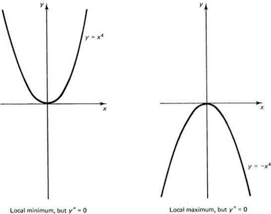
Figure 8.6-6
Another way of saying things is:
1.y′ = 0, y″ > 0 implies a local minimum
2.y′ = 0, y″ < 0 implies a local minimum
3.y′ = 0, y″ = 0 implies no conclusion
Example 8.6-2
Find the zeros and the inflection points of
![]()
Note first that the curve has odd symmetry, f(x, y) =f(–x, –y). To find the zeros, we start to factor it. There is a factor of x, and the rest is a quadratic in x2. Therefore,
![]()
The zeros are easily seen to be ![]() and
and ![]() .
.
To find the inflection points, differentiate twice (almost directly term by term) and equate to zero:
![]()
Divide out the common factor 60 to leave
![]()
whose zeros are – 1, 0, and 1. The function values at these points are already known to be zero! This function has inflection points and zeros at the same three points, –1,0, and 1 (and has a pair of other zeros). We are ready to sketch it, except that we have no value to give the scale in the y direction. If we put x = 2 in the factored form of the polynomial, we get
y = 2(3)(5) = 30
and if we use x = ![]() we get
we get
![]()
To find the maximum and minimum, we have the equation
![]()
(which is a quadratic in x2), whose zeros are given by
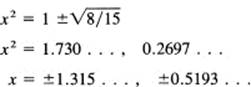
The square roots are taken to get the x values. It is less difficult to handle when you recognize that x2 occurs frequently in the evaluation of the equation written in the form
y = x(3x4 – 10x2 + 7)
With a hand calculator, it is easy to place the points where the local extremes occur. The sketch is shown in Figure 8.6-7.
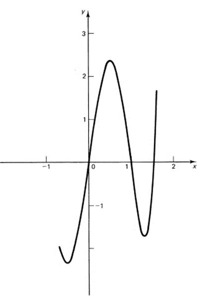
Figure 8.6-7 y = 3x5 – 10x3 + 7x
EXERCISES 8.6
1.Find the distance between the inflection points of y = 1/(1 + x2).
2.Find the slope at the inflection points of the above equation.
3.Find the zeros, maximum, minimum and inflection points of y = x5 – 2x3 + x.
8.7 CURVE TRACING
It is essential to learn to sketch the curve of a given function. It is an art to do it easily and gracefully. The most useful tool is symmetry, because each form of symmetry decreases the work by about a factor of 2. Let us review the simple rules from Section 6.11. They were based, as you remember, on invariance of the equation under substitutions of the variables.
1.Symmetry with respect to the x-axis. Typical terms that have this property are constants, y2, y4, …, |y|, cos y, and so on. The rule is: functions that are of even degree in y are symmetric with respect to the x-axis. Replacing y by –y does not change the equation.
2.Symmetry with respect to the y-axis. Same as above except x in place of y. Replacing x by –x does not change the equation.
3.Symmetry with respect to the origin. Typical terms, xy, (xy)2, … , sin x sin y, cos x, cos y, x2 + y2, … , and so on. Replacing both x and –x and y by –y does not change the equation.
Note that if you have two of the above you automatically have the third.
4.Odd symmetry. The same as above (3) ; the function on one side of the origin is the negative of the function on the other. Typical terms are odd powers of x in place of even powers, sines or tangents in place of cosines, and so on. Clearly, “symmetry” means “even symmetry” unless specifically it is said to be “odd symmetry.”
5.Symmetry with respect to the 45° line. Typical terms, xy, (xy)2, …, x + y, x2 + y2, …, and so on. In words, nothing happens when you interchange x and y in the equation.
As we said, do not try to learn all the above rules, but rather in such a situation ask, “What is behind all this complexity?” A little thought shows that it is the invariance of the equation under the appropriate substitutions. For example, the equation
x2 + y2 = a2
is not changed by replacing x by –x. Hence any point (x, y) that satisfies the equation has the corresponding point (-x, y). What does this mean? The same y value but opposite x values; symmetry with respect to the y-axis. Thus the mathematician learns to inspect a given equation for invariances of all kinds, and when one is found it is often easily exploitable. Once having thought your way through various invariances to their symmetries, you need only recall the method, not memorize the long list of results. Some invariances are harder to interpet because they are not symmetries. For example, the equation
![]()
has the change of variables x→l/x and y→1/y that leaves the equation invariant. The meaning of the invariance is more complicated than simple symmetry. But each invariance cuts down the difficulty of plotting points by a factor of about 2.
Another tool for curve tracing is the choice of a few values of x for which it is easy to get values of y. When you are given y = f(x), it is easy to compute pairs of values that satisfy the function. In cases where you cannot easily solve for either of the variables in terms of the other, you must guess at likely pairs of values.
Next, you have the maximum and minimum points. Not only do you need the x values, but also the corresponding y values (if you can get them easily). The maximum and minimum points greatly constrain the function’s behavior.
Next, you have the inflection points. Again, you need the corresponding y values (if you can get them). Often the slope of the curve at the inflection points greatly aids in sketching the curve.
Finally, you have those particular values for which x or y, or both, go to infinity. When these are used, or at least some of them, you have a fairly good idea of what the curve does far away from the origin. This kind of information can help, even when you are near the origin.
The importance and usefulness of curve tracing cannot be overemphasized. On a number of occasions a simple sketch on the back of a luncheon placemat has answered important technical questions.
In curve tracing it is an art to do those things that come easily, and not to use those that are hard. All we can do is give a few examples to illustrate curve tracing, followed by some personal practice by you. Remember, the purpose of the exercises is not to get the answer but rather to learn the art.
Example 8.7-1
Sketch the curve
x2y2 = a4
Clearly, there is a scale to the figure; we really need to think of the transformation of x to ax1 and y to ay1. Then the a4 would cancel out. Thus, we temporarily replace a by 1 for convenience, and in the final drawing (but not necessarily along the way) we plot in units of size a.
As for symmetry, the even powers in both variables show that we have symmetry with respect to the x-axis, the y-axis, and the origin. Thus it suffices to examine the first quadrant and then suitably duplicate it for the other quadrants. In the first quadrant we examine the curve
x2y2 = 1
and, because the quantities are positive, we can take the square root of each side. We recognize the hyperbola (in the first and third quadrants)
xy = 1
There is, of course, a second equation with a minus sign. To get the scale, we note that the point x = 1, y = 1 lies on the curve. It is also easy to find the points x = 2, y = ![]() and x =
and x = ![]() y = 2 on the curve. Thus the full sketch is in Figure 8.7-1.
y = 2 on the curve. Thus the full sketch is in Figure 8.7-1.
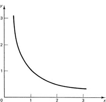
Figure 8.7-1 x2y2 = 1
Example 8.7-2
Another example is
![]()
We see immediately that there are only even powers of x, and hence symmetry with respect to the y-axis. Next, the zeros of the function are at x = –1 and 1. At the point x = 0, the curve has the value y = – 1.
The derivative
![]()
gives only one value for an extreme, that is, at x = 0. The function value at this place is, again, –1; it looks like a local minimum. The numerator of the second derivative (which is usually all we need) is
![]()
from which we deduce that at the x values ![]() are the inflection points. The corresponding function values are easily found to be
are the inflection points. The corresponding function values are easily found to be
![]()
It remains to see what happens far from the origin. For large absolute x values, the y values approach 1 from below. There can be no large y values (apparently, but you can be fooled if you are too hasty in thinking!). A final point x = 2, y = ![]() helps nail down the curve.
helps nail down the curve.
We are ready for the sketch. At x = 0 we begin at y = –1 with y′ = 0. It is concave up until ![]() , where the y value is –
, where the y value is –![]() . Continuing, it must be concave down and pass through x = 1, where y = 0. It continues to rise slowly, passing through the point x = 2,
. Continuing, it must be concave down and pass through x = 1, where y = 0. It continues to rise slowly, passing through the point x = 2, ![]() and is limited far out by y = 1 (see Figure 8.7-2). Symmetry gives the curve for negative x.
and is limited far out by y = 1 (see Figure 8.7-2). Symmetry gives the curve for negative x.
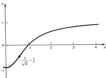
Figure 8.7-2 ![]()
Example 8.7-3
Plot the family of curves (n ≥ 1)
x2n + y2n = a2n
Evidently, the change of variables ax → x, ay → y will remove the parameter a. Hence we can act as if a = 1 and at the last moment put units of a on the axes.
For n = 1, the equation is a circle. For n = 2, we have
x4 + y4 = 1
to think about. Since numbers smaller than 1 in size when raised to a high power become smaller, it will require larger numbers than for the circle to satisfy the equation. To find out how large, we look along the 45° line along which x = y. There we find we have
![]()
Thus we see that it looks somewhat like a circle but “bulges out” a bit.
For the next case, n = 3, the similar point is the solution
![]()
and so on. In the limit as n → ∞, we have the curve approaching the square containing the original circle (see Figure 8.7-3).
Sometimes the curves you wish to understand have several parameters and cannot be plotted for any definite values without the risk of losing some information.
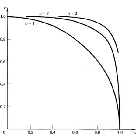
Figure 8.7-3 x2n + y2n = 1
You need to be able to plot in your imagination, and then prove, that all possible values have a given property, as the following example shows.
Abstraction 8.7-4
Can we see the previous family of curves from a unified viewpoint? If we can, then we have a great diversity mastered under a single form for reference, something you should always try to do.
The exponent = 2 is the familiar circle. How does the exponent 2 arise? It comes from the Pythagorean definition of the distance between two points. But suppose you defined the distance between two points as
![]()
You would then have “circles” about the origin (0, 0) in all finite cases of the exponent.
But is that a reasonable definition of a distance? In Section 5.2 we gave the following conditions:
1.d(p1, p2) ≥ 0
2.d(p1, p2) = 0 if and only if p1 = p2
3.d(p1, p2) = d(p2, p1)
4.d(p1, p2) + d(p2,p3)≥ d(p1, p3)
Does the generalized distance have these properties? Looking at the exponent = 1, called Li (“ell one”), we see that the distance
![]()
is simply the sum of the absolute values of the differences. It is as if you had to go along the sides and there were no diagonals when you measured distances. In this distance the circle is the square-shaped diamond shown in Figure 8.7-4.
We see from the earlier curves that as n gets larger the corresponding circles bulge out and approach the square in the limit. This limit is called L∞ (“ell infinity,” or sometimes the Chebyshev distance). The distance is given by the formula
![]()
as you can see when you look at how the large exponents used tend to select out the largest term at the expense of all other possible terms. The corresponding root brings that term back to its original size.
It is not hard to see that by algebra alone the first three conditions for a distance are true. The fourth condition comes at present from your intuition.
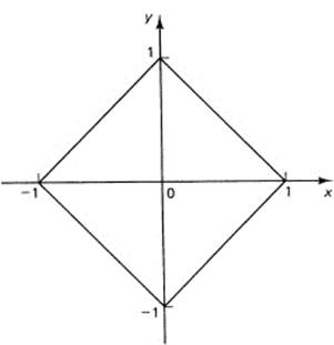
Figure 8.7-4 |x| + |y| = 1
Example 8.7-5
Discriminant of a cubic. One day, when I had no textbooks handy, I needed to know when a cubic
ax3 + bx2 + cx + d = 0
has all real roots. I recalled (and checked by carrying it out) that this could be reduced to a simpler form by the substitution
![]()
which you can see eliminates the square term. The reduced cubic form (which is usually presented in the variable y) is
y3+ py + q = 0
A typical shape of a cubic is shown in Figure 8.7-5. The wiggles are characteristic, but do not always occur. If the equation is to have three real roots, then the minimum must be a negative number, and the maximum a positive number; otherwise there will not be three crossings. These two conditions can be combined into one by calling the cubic P(y) and writing
P(ymin)P(ymax) < 0
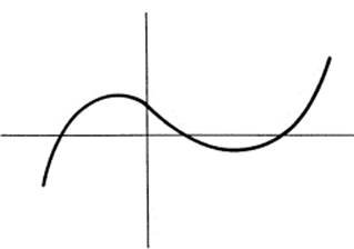
Figure 8.7-5 Cubic
What about the equality? Yes, when either of the extremes is zero, there is a double (real) root, and if both are zero, then it is clearly the triple root of the equation y3 = 0. Hence we take
P(ymin)P(ymax) ≤ 0
as the test.
We have, therefore, to compute this quantity. The derivative of the cubic, when set equal to zero, gives the position of the extremes:
![]()
Hence ![]() and
and ![]() . We have, therefore, on setting (p must be negative for real solutions)
. We have, therefore, on setting (p must be negative for real solutions)
![]()
to compute
![]()
This becomes, on eliminating the R,
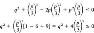
This can be rewritten in the more easily remembered form
![]()
which is the conventional discriminant of the cubic and is the condition for three real roots.
EXERCISES 8.7
1. Examine the family ![]()
8.8 FUNCTIONS, EQUATIONS, AND CURVES
In Section 4.3 we defined a function as a relationship such that given an x (in some range) there is a unique value y corresponding to it. Generally, we deal with functions that can be expressed by equations (although not always!).
But an equation is not always a function. Thus the equation for a circle
x2 + y2 = a2
is not a function, but leads to two functions
![]()
for |x| < a.
When we examined the family of curves
|x|n + |y|n = an
we found various shapes depending on the exponent n. We also looked at the limit as n →∞. There we had a curve, but no equation—only the limit of an equation.
We see, therefore, that if we want to be careful we need to realize that the three concepts, function, equation, and curve, are not all exactly the same.
8.9 SUMMARY
The geometric applications of the calculus are very important. Tangent and normal lines are needed tools in many situations and lead naturally to curvature and convexity. These in turn lead to the max-min test for local extremes in the interval. It is not necessary to dwell on the importance of optimization in most fields since it is a natural question to ask in many situations.
The art of curve tracing is an important talent to master; in many complex situations it enables you to “see” what you are examining. Sketches are much more easily grasped by the human mind than are long tables of numbers, or even mathematical equations. It should be noted, however, that, when a parameter occurs in an equation, the equation may be more revealing than a lot of curves!
This chapter is a tool kit of useful methods for dealing with the world. Each tool should be recognized as a “chunk” of knowledge. You should review them in your mind until they are seen as units of thought, and not as individual complex patterns of details. Of course, you must also see the details when you focus on the particular tool. Mastery of a topic implies both the “chunking” and the ability, when needed, to call up the relevant details of the “chunk.”