Mathematics, Substance and Surmise: Views on the Meaning and Ontology of Mathematics (2015)
From the continuum to large cardinals
John Stillwell1
(1)
Mathematics Department, University of San Francisco, 2130 Fulton Street, San Francisco, CA 94117, USA
John Stillwell
Email: stillwell@usfca.edu
Abstract
Continuity is one of the most important concepts of mathematics and physics. This has been recognized since the time of Euclid and Archimedes, but it has also been understood that continuity raises awkward questions about infinity. To measure certain geometric quantities, such as the diagonal of the unit square, or the area of a parabolic segment, involves infinite processes such as forming an infinite sum of rational numbers. For a long time, it was hoped that “actual” infinity could be avoided, and that the necessary uses of infinity could be reduced to “potential” form, in which infinity is merely approached, but never reached. This hope vanished in the 19th century, with discoveries of Dedekind and Cantor. Dedekind defined the points on the number line via infinite sets of rational numbers, and Cantor proved that these points form an uncountable infinity—one that is actual and not merely potential. Cantor’s discovery was part of his theory of infinity that we now call set theory, at the heart of which is the discovery that most of the theory of real numbers, real functions, and measure takes place in the world of actual infinity. So, actual infinity underlies much of mathematics and physics as we know it today. In the 20th century, as Cantor’s set theory was systematically developed, we learned that the concept of measure is in fact entangled with questions about the entire universe of infinite sets. Thus the awkward questions raised by Euclid and Archimedes explode into huge questions about actual infinity.
1 Introduction
The real number system ![]() , traditionally called the continuum, has been a mystery and a spur to the development of mathematics since ancient times. The first important event in this development was the discovery that
, traditionally called the continuum, has been a mystery and a spur to the development of mathematics since ancient times. The first important event in this development was the discovery that ![]() is irrational; that is, not a ratio of whole numbers. This discovery led to the realization that measuring (in this case, measuring the diagonal of the square) is a more general task than counting, because there is no unit of length that allows both the side and the diagonal of the square to be counted as integer multiples of the unit.
is irrational; that is, not a ratio of whole numbers. This discovery led to the realization that measuring (in this case, measuring the diagonal of the square) is a more general task than counting, because there is no unit of length that allows both the side and the diagonal of the square to be counted as integer multiples of the unit.
Thus, by around 300 BCE, when Greek mathematics was systematized in Euclid’s Elements, there was a clear distinction between the theory of magnitudes (measuring length, area, and volume) and the theory of numbers (whole numbers and their arithmetic). The former was handled mainly by geometric methods; the latter was like the elementary number theory of today, and its characteristic method of proof was induction. Euclid did not recognize induction as an axiom, but he used it—in the form we now call well-ordering—to prove crucial results. For example, in the Elements, Book VII, Proposition 31, he uses induction to prove that any composite number n is divisible by a prime as follows.
Given that n = ab, for some positive integers a, b < n, if either a or b is prime we are done; if not, repeat the argument with a. This process must eventually end with a prime divisor of n. If not, we get an infinite decreasing sequence of positive integers which, as Euclid says, “is impossible in numbers.”
Thus Euclid is using the principle that any decreasing sequence (of positive integers) is finite, which is what we now call the well-ordering property of the positive integers.
Euclid’s theory of magnitudes is evidently something more than his theory of numbers, since it covers magnitudes such as ![]() , but it is hard to pinpoint the extra ingredient, because Euclid’s axioms are sketchy and incomplete by modern standards. (Nevertheless, they served mathematics well for over two millenia, setting a standard for logical rigor that was surpassed only in the 19th century.) The relationship between the theory of magnitudes and the theory of numbers was developed in Book V of the Elements, a book whose subtlety troubled mathematicians until the 19th century. Although the details of Book V are complicated, its basic idea is simple: compare magnitudes (our real numbers) by comparing them with rational numbers. That is
, but it is hard to pinpoint the extra ingredient, because Euclid’s axioms are sketchy and incomplete by modern standards. (Nevertheless, they served mathematics well for over two millenia, setting a standard for logical rigor that was surpassed only in the 19th century.) The relationship between the theory of magnitudes and the theory of numbers was developed in Book V of the Elements, a book whose subtlety troubled mathematicians until the 19th century. Although the details of Book V are complicated, its basic idea is simple: compare magnitudes (our real numbers) by comparing them with rational numbers. That is
![]()
The power of this idea was not fully realized until 1858, when Dedekind used to give the first rigorous definition of the continuum.
In the meantime, the intuition of the continuum had developed and flourished since the mid-17th century. Newton based the concepts of calculus on the idea of continuous motion, and the subsequent development of continuum mechanics exploited the continuum of real numbers (and its higher-dimensional generalizations) as a model for all kinds of continuous media. This made it possible to study the behavior of vibrating strings, fluid motion, heat flow, and elasticity. Almost the only exception to continuum modeling before the 20th century was Daniel Bernoulli’s kinetic theory of gases (1738, with extensions by Maxwell and Boltzmann in the 19th century), in which a gas is modeled by a large collection of particles colliding with each other and the walls of a container. Even there, the underlying concept was continuous motion, since each particle was assumed to move continuously between collisions.
Thus, long before the continuum was well understood, it had become indispensable in mathematics.
The understanding of the continuum finally advanced beyond Euclid’s Book V in 1858, when Dedekind extended the idea of comparing x and y via rational numbers to the idea of determining x (or y) via rational numbers. But while we can separate x from y finding just one rational number m∕n strictly between them, to determine x we need to separate (or cut) the whole set of rational numbers into those less than x and those greater than x. Thus the exact determination of an irrational number x requires infinitely many rational numbers, say those greater than x. For example, ![]() is determined by the set of positive rational numbers m∕n such that
is determined by the set of positive rational numbers m∕n such that ![]() .
.
Although Dedekind’s concept of a cut in the rational numbers is a logical extension of the ancient method for comparing two lengths, it is not a step that the Greeks would have taken, because they did not accept the concept of an infinite set. In determining real numbers by infinite sets of rational numbers, Dedekind brought to light the fundamental role of infinity in mathematics. In a sense we will make precise later, mathematics can be defined as “elementary number theory plus infinity.” But before doing so (and before deciding “how much” infinity we need), let us examine more closely what we want from the continuum.
2 What does the Continuum Do for Mathematics?
The immediate effect of Dedekind’s construction of the continuum was to unify the ancient geometric theory of magnitudes with the arithmetic theory of numbers in a number line. Certainly, mathematicians for centuries had assumed there was such a thing, but Dedekind was the first to define it and to prove that it had the required geometric and arithmetic properties: numbers fill the line without gaps and they can be added and multiplied in a way that is compatible with addition and multiplication of rational numbers.
As a consequence, we get the basic concepts of the theory of measure: length, area, and volume. The length of the interval [a, b] from a to b is b − a; the area of a rectangle of length l and width w is lw; the volume of a box of length l, width w, and depth d is lwd. Today, we take it for granted that the area or volume of a geometric figure is simply a number, but this is not possible until there is a number for each point on the line.1
The absence of gaps in ![]() , which we now call completeness, was called continuity by Dedekind. Indeed, Dedekind’s continuous line is a precursor to the modern concept of continuous curve (in the plane, say) which is defined by a continuous function from the line or an interval of the line into the plane. Such a curve has no gaps because the line has none. Another consequence of the “no gaps” property is the intermediate value theorem for continuous functions: if f is continuous on an interval [a, b] and f(a) and f(b) have opposite signs, then f(c) = 0 for some c between a and b. Other basic theorems about continuous functions also depend on the completeness of
, which we now call completeness, was called continuity by Dedekind. Indeed, Dedekind’s continuous line is a precursor to the modern concept of continuous curve (in the plane, say) which is defined by a continuous function from the line or an interval of the line into the plane. Such a curve has no gaps because the line has none. Another consequence of the “no gaps” property is the intermediate value theorem for continuous functions: if f is continuous on an interval [a, b] and f(a) and f(b) have opposite signs, then f(c) = 0 for some c between a and b. Other basic theorems about continuous functions also depend on the completeness of ![]() . In fact, it was to provide a sound foundation for such theorems of analysis that Dedekind proposed a definition of
. In fact, it was to provide a sound foundation for such theorems of analysis that Dedekind proposed a definition of ![]() in the first place.
in the first place.
With this foundation established, all the applications of analysis to continuum mechanics, mentioned in the previous section, become soundly based as well. The continuum also meets other needs of analysis, because its completeness implies that various infinite processes on ![]() lead to a result whenever they ought to. For example, an infinite sequence of real numbers
lead to a result whenever they ought to. For example, an infinite sequence of real numbers
![]()
has a limit if and only if it satisfies the Cauchy criterion: for all ![]() there is an N such that
there is an N such that
![]()
With the help of the limit concept we can make sense of infinite sums ![]() of real numbers. Namely, if
of real numbers. Namely, if ![]() , then
, then ![]() is the limit of the sequence
is the limit of the sequence ![]() , if it exists.
, if it exists.
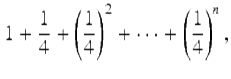
Infinite sums are also important in geometry. Special cases were used (implicitly) by Euclid and Archimedes to determine areas and volumes. A wonderful example is the way Archimedes determined the area of a parabolic segment by dividing it into infinitely many triangles, as indicated in Figure 1.In modern language, this is the segment of the parabola y = x 2 between ![]() and x = 1. The first approximation to its area is the black triangle, which has area 1. The second approximation is obtained by adding the two dark gray triangles, which have total area 1/4. The third is obtained by adding the four light gray triangles, which have total area (1∕4)2, and so on.
and x = 1. The first approximation to its area is the black triangle, which has area 1. The second approximation is obtained by adding the two dark gray triangles, which have total area 1/4. The third is obtained by adding the four light gray triangles, which have total area (1∕4)2, and so on.
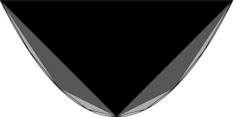
Fig. 1
Filling the parabolic segment with triangles
It is clear that by taking enough triangles we can approach the area of the parabolic segment arbitrarily closely, and it can also be shown (by the formula for the sum of a geometric series) that
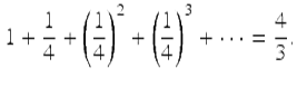
Thus the area being approached in the limit—the area of the parabolic segment—is 4/3. It is a happy accident in this case that the area turns out to be expressible by a geometric series, which we know how to sum. In other cases we can exploit the geometric series to prove that certain sets of points have zero length or area.
For example, let ![]() be any subset of
be any subset of ![]() whose members can be written in a sequence. I claim that S has zero length. This is because, for any
whose members can be written in a sequence. I claim that S has zero length. This is because, for any ![]() , we can cover S by intervals of total length
, we can cover S by intervals of total length ![]() . Namely,
. Namely,
cover x 1
by an interval of length ![]() ,
,
cover x 2
by an interval of length ![]() ,
,
cover x 3
by an interval of length ![]() , and so on.
, and so on.
In this way, each point of S is covered, and the total length of the covering is at most
![]()
Thus the length of S is ![]() , for any
, for any ![]() , and so the length of S can only be zero.
, and so the length of S can only be zero.
This innocuous application of the geometric series has two spectacular consequences:
1.
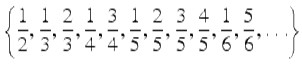
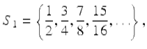
The set of rational numbers between 0 and 1 has total length zero, because these numbers can be written in the sequence
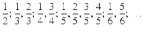
(taking all those with denominator 2, then those with denominator 3, and so on). It follows that the rational numbers do not include all the numbers between 0 and 1, which gives another proof that irrational numbers exist.
2.
The real numbers between 0 and 1 cannot be written in a sequence. We say that there are uncountable many real numbers between 0 and 1. It follows that ![]() itself is uncountable.2
itself is uncountable.2
Thus the theory of measure, which ![]() makes possible, tells us something utterly unexpected: uncountable sets exist, and
makes possible, tells us something utterly unexpected: uncountable sets exist, and ![]() is one of them. In fact, the theory of measure brings to light even more unexpected properties of infinity, as we will see, but first we should take stock of the implications of uncountability.
is one of them. In fact, the theory of measure brings to light even more unexpected properties of infinity, as we will see, but first we should take stock of the implications of uncountability.
3 Potential and Actual Infinity
When Archimedes found the area of the parabolic segment by dividing it into infinitely many triangles he did not argue precisely as I did in the previous section. He did not sum the infinite series
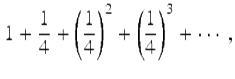
but only the finite series
which has sum ![]() . This makes little practical difference, since the finite collection of triangles being measured approaches the parabolic segment in area, and the numerical value of the area clearly approaches 4/3. However, there was a conceptual difference that was important to the Greeks: only finite sets need be considered.
. This makes little practical difference, since the finite collection of triangles being measured approaches the parabolic segment in area, and the numerical value of the area clearly approaches 4/3. However, there was a conceptual difference that was important to the Greeks: only finite sets need be considered.
The Greeks invariably avoided working with infinite sets when it was possible to work with finite sets instead, as is the case here. The avoidable infinite sets are those we now call countably infinite. As the name suggests, an infinite set is countable if we can arrange its members in a list
![]()
so that each member occurs at some finite position. The prototype countable set is the set ![]() of positive integers. Indeed, another way to say that an infinite set is countable is to say that there is a one-to-one correspondence between its members and the members of
of positive integers. Indeed, another way to say that an infinite set is countable is to say that there is a one-to-one correspondence between its members and the members of ![]() . Another countably infinite set that we have already seen is the set
. Another countably infinite set that we have already seen is the set
of rational numbers between 0 and 1.
The Greeks, and indeed almost all mathematicians until the 19th century, believed that countably infinite sets existed in only a potential, rather than actual, sense. An infinite set is one whose members arise from a process of generation, and one should not imagine the process being completed because it is necessarily endless. Likewise, a convergent infinite sequence is a process that grows toward the limiting value, without actually reaching it. Mathematicians issued stern warnings against thinking of infinity in any other way. An eminent example was Gauss, who wrote in a letter to Schumacher (12 July 1831) that:
I protest against the use of infinite magnitude as something completed, which is never permissible in mathematics. Infinity is merely a way of speaking, the true meaning being a limit which certain ratios approach indefinitely closely, while others are permitted to increase without restriction.
As long as it was possible to avoid completed infinities, then of course it seemed safer to reject them. But it ceased to be possible when Cantor discovered the uncountability of ![]() in 1874. Since
in 1874. Since ![]() is uncountable, it is impossible to view it as the unfolding of a step-by-step process, as
is uncountable, it is impossible to view it as the unfolding of a step-by-step process, as ![]() unfolds from 1 by repeatedly adding 1. For better or for worse, we are forced to view
unfolds from 1 by repeatedly adding 1. For better or for worse, we are forced to view ![]() as a completed whole.
as a completed whole.
Cantor’s first uncountability proof was not the measure argument given in the previous section, but one related to Dedekind’s idea of separating sets of rationals into upper and lower parts. In 1891 Cantor discovered a new, simpler, and more general argument that leads to an unending sequence of larger and larger infinities. This is the famous diagonal argument, which shows that any set X has more subsets than members.
Suppose that, for each x ∈ X, we have a subset ![]() . Thus we have “as many” subsets as there are members of X. It suffices to show that the sets S x do not include all subsets of X. Indeed, they do not include the subset
. Thus we have “as many” subsets as there are members of X. It suffices to show that the sets S x do not include all subsets of X. Indeed, they do not include the subset
![]()
because D differs from each S x with respect to the element x.
An important consequence of the diagonal argument is that there is no largest set. This is because, for any set X, there is the larger set ![]() whose members are the subsets of X.
whose members are the subsets of X.
The reason for calling Cantor’s argument “diagonal” becomes apparent if we take the case ![]() . Then subsets
. Then subsets ![]() of
of ![]() may then be encoded as rows of 0s and 1s in an infinite table like that shown in Figure 2, where a 1 in column n says that n is a member, and 0 in column n says that n is not a member. Thus, in the table shown, S 1 is the set of even numbers, S 2 is the set of squares, and S 3 is the set of primes. The diagonal digits (shown in bold) say whether or not n ∈ S n , and we construct D by switching each of these digits, so n ∈ D if and only if n ∉ S n .
may then be encoded as rows of 0s and 1s in an infinite table like that shown in Figure 2, where a 1 in column n says that n is a member, and 0 in column n says that n is not a member. Thus, in the table shown, S 1 is the set of even numbers, S 2 is the set of squares, and S 3 is the set of primes. The diagonal digits (shown in bold) say whether or not n ∈ S n , and we construct D by switching each of these digits, so n ∈ D if and only if n ∉ S n .
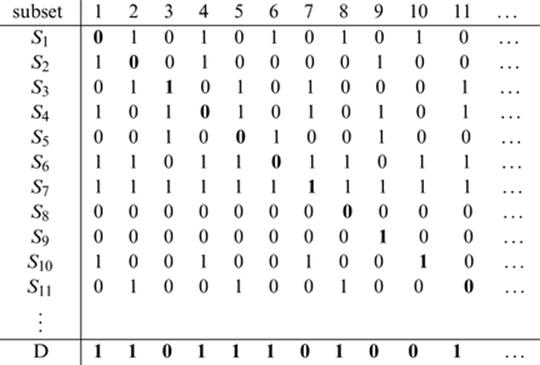
Fig. 2
The diagonal argument
The set ![]() is in fact “of the same size” as
is in fact “of the same size” as ![]() , because there is a one-to-one correspondence between infinite sequences of 0s and 1s and real numbers. Such a correspondence can be set up using binary expansions of real numbers, but we skip the details, which are somewhat messy.
, because there is a one-to-one correspondence between infinite sequences of 0s and 1s and real numbers. Such a correspondence can be set up using binary expansions of real numbers, but we skip the details, which are somewhat messy. ![]() is just one of several interesting sets of the same size (or same cardinality, to use the technical term) as
is just one of several interesting sets of the same size (or same cardinality, to use the technical term) as ![]() . Another is the set
. Another is the set ![]() of points in the plane, and an even more remarkable example is the set of continuous functions from
of points in the plane, and an even more remarkable example is the set of continuous functions from ![]() to
to ![]() . Thus all of these sets are uncountable, and hence not comprehensible as merely “potential” infinities.
. Thus all of these sets are uncountable, and hence not comprehensible as merely “potential” infinities.
4 The Unreasonable Effectiveness of Infinity
In 1949, Carl Sigman and Bob Russell wrote the jazz standard “Crazy he calls me,” soon to be made famous by Billie Holliday. Its lyrics include the lines
The difficult I’ll do right now
The impossible will take a little while
A mathematical echo of these lines is a saying attributed to Stan Ulam:
The infinite we shall do right away.
The finite may take a little longer.
I do not know a direct source for this quote, or what Ulam was referring to, but it captures a common experience in mathematics. Infinite structures often arise more naturally, and are easier to work with than their finite analogues.
The continuum is a good example of an infinite structure that is easier to work with than any finite counterpart, perhaps because there is no good finite counterpart. Even when one is forced to work with a finite instrument, such as a digital computer, it is easier to have an underlying continuum model, such as ![]() in the case of robotics, as Ernest Davis has explained in his chapter.
in the case of robotics, as Ernest Davis has explained in his chapter.
In the history of mathematics there are many cases where ![]() helps, in a mysterious way, to solve problems about finite objects. There are theorems about natural numbers first proved with the help of
helps, in a mysterious way, to solve problems about finite objects. There are theorems about natural numbers first proved with the help of ![]() , and theorems about
, and theorems about ![]() that paved the way for analogous (but more difficult) theorems about finite objects.
that paved the way for analogous (but more difficult) theorems about finite objects.
An example of the former type is Dirichlet’s 1837 theorem on primes in arithmetic progressions: if a and b are relatively prime, then the sequence
![]()
contains infinitely many primes. Dirichlet proved this theorem with the help of analysis, and it was over a century before an “elementary” proof was found, by Selberg in 1948. Even now, analytic proofs of Dirichlet’s theorem are preferred, because they are shorter and seemingly more insightful.
An example of the latter type is the classification of finite simple groups, the most difficult theorem yet known, whose proof is still not completely published. An infinite analogue of this theorem, the classification of simple Lie groups, was discovered by Killing in 1890. It is likely that the classification of finite simple groups would not have been discovered without Killing’s work, because it required the insight that many finite groups are analogues of Lie groups, obtained by replacing ![]() by a finite field.
by a finite field.
Thus, for reasons we do not really understand, ![]() gives insight and brings order into the world of finite objects. Is it also possible that some higher infinity brings insight into the world of
gives insight and brings order into the world of finite objects. Is it also possible that some higher infinity brings insight into the world of ![]() ? The answer is yes, and in fact we understand better how higher infinities influence the world of
? The answer is yes, and in fact we understand better how higher infinities influence the world of ![]() than how
than how ![]() influences the world of natural numbers. The surprise is just how “large” the higher infinities need to be. To explain what we mean by “large,” we first need to say something about axioms of set theory.
influences the world of natural numbers. The surprise is just how “large” the higher infinities need to be. To explain what we mean by “large,” we first need to say something about axioms of set theory.
5 Axioms of Set Theory
The idea that sets could be the foundation of mathematics developed in the 19th century. Originally their role was thought to be quite simple: there were numbers, and there were sets of numbers, and that was sufficient to define everything else (this was when “everything” was based on ![]() ). But then in 1891 the set concept expanded alarmingly when Cantor discovered the endless sequence of cardinalities produced by the power set operation
). But then in 1891 the set concept expanded alarmingly when Cantor discovered the endless sequence of cardinalities produced by the power set operation ![]() . It follows that there is no largest set, as we saw in Section 3, and hence there is no set of all sets. For some mathematicians (Dedekind among them) this was alarming and paradoxical because it implies that not every property defines a set. In particular, the objects X with the property “X is a set” do not form a set.
. It follows that there is no largest set, as we saw in Section 3, and hence there is no set of all sets. For some mathematicians (Dedekind among them) this was alarming and paradoxical because it implies that not every property defines a set. In particular, the objects X with the property “X is a set” do not form a set.
However, there is a commonsense way to escape the paradox, first proposed by Zermelo in 1904. Just as the natural numbers are generated from 0 by the operation of successor, and there is no “number of all numbers” because every number has a successor, sets might be generated from the empty set ∅ by certain operations, such as the power set operation. With this approach to the set concept there is no “set of all sets” because every set X has a power set ![]() , which is larger.
, which is larger.
Thus Zermelo began with the following two axioms, which state the existence of ∅ and the definition of equality for sets:
Empty Set.
There exists a set ∅ with no members.
Extensionality.
Sets are equal if and only if they have the same members.
All other sets are generated by the following set construction axioms.
Pairing.
For any sets A, B there is a set {A, B} whose members are A and B. (If A = B, then {A, B} = { A, A}, which equals {A} by Extensionality.)
Union.
For any set X there is a set ![]() whose members are the members of members of X. (For example, if X = { A, B}, then
whose members are the members of members of X. (For example, if X = { A, B}, then ![]() .)
.)
Definable Subset.
For any set X, and any property ![]() definable in the language of set theory, there is a set
definable in the language of set theory, there is a set ![]() whose members are the members of X with property
whose members are the members of X with property ![]() .
.
Power Set.
For any set X there is a set ![]() whose members are the subsets of X.
whose members are the subsets of X.
These axioms produce enough sets to play the role of all mathematical objects in general use. In particular, the natural numbers ![]() may be elegantly realized as follows:
may be elegantly realized as follows:
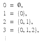
This definition, proposed by von Neumann in 1923, has the bonus features that the < relation between numbers is simply the membership relation ∈ , and the successor function is ![]() . With the help of an“induction” axiom, which we postpone until the next section, it is possible to develop all of the elementary theory of numbers from these axioms. However, we cannot yet prove the existence of infinite sets. Infinity has to be introduced by another axiom.
. With the help of an“induction” axiom, which we postpone until the next section, it is possible to develop all of the elementary theory of numbers from these axioms. However, we cannot yet prove the existence of infinite sets. Infinity has to be introduced by another axiom.
Infinity.
There is a set I whose members include ∅ and, along with each member x, the member ![]() .
.
It follows that I has all the natural numbers ![]() as members, and the property of being a natural number is definable, so we can obtain the set
as members, and the property of being a natural number is definable, so we can obtain the set ![]() as a definable subset of I. Finally, we can use Power Set and Pairing to obtain the real numbers from
as a definable subset of I. Finally, we can use Power Set and Pairing to obtain the real numbers from ![]() via Dedekind cuts, and hence obtain the set
via Dedekind cuts, and hence obtain the set ![]() .
.
A useful trick here and elsewhere is to define the ordered pair (a, b) as {{a}, {a, b}}. Among their other uses, ordered pairs are crucial for the definition of functions, which can be viewed as sets of ordered pairs.
The universe of sets obtained by the Zermelo axioms is big enough to include all the objects of classical mathematics; in fact, most classical objects are probably included in ![]() . Nevertheless, it is easy to imagine sets that fall outside the Zermelo universe. One such set is
. Nevertheless, it is easy to imagine sets that fall outside the Zermelo universe. One such set is
![]()
obtained by repeating the power set operation indefinitely and taking the union of all the resulting sets. U cannot be proved to exist from the Zermelo axioms. For this reason, Fraenkel in 1922 strengthened Definable Subset to the following axiom.
Replacement.
If X is a set and if ![]() is a formula in the language of set theory that defines a function y = f(x) with domain X, then the range of f,
is a formula in the language of set theory that defines a function y = f(x) with domain X, then the range of f,
![]()
is also a set.
With this axiom, the set U can be proved to exist, because we can define
![]()
as the range of a function ![]() on
on ![]() , and then obtain U as
, and then obtain U as ![]() .
.
The above axioms, together with the “induction” axiom to be discussed in the next section, form what is now called Zermelo-Fraenkel set theory, or ZF for short. Its language, which was presupposed in the Definable Subset and Replacement axioms can very easily be made precise. It contains the symbols ∈ and = for membership and equality, letters ![]() for variables, parentheses, and logic symbols. ZF is a plausible candidate for a system that embraces all of mathematics, because there are no readily imagined sets that cannot be proved to exist in ZF. Nevertheless, we find ourselves drawn beyond ZF when we try to resolve certain natural questions about
for variables, parentheses, and logic symbols. ZF is a plausible candidate for a system that embraces all of mathematics, because there are no readily imagined sets that cannot be proved to exist in ZF. Nevertheless, we find ourselves drawn beyond ZF when we try to resolve certain natural questions about ![]() .
.
6 Set Theory and Arithmetic
Before investigating what ZF can prove about ![]() , it is worth checking whether ZF can handle elementary number theory. We have already seen that, without even using the axiom of Infinity, we can define the natural numbers
, it is worth checking whether ZF can handle elementary number theory. We have already seen that, without even using the axiom of Infinity, we can define the natural numbers ![]() , the < relation, and the successor function
, the < relation, and the successor function ![]() . This paves the way for inductive definitions of addition and multiplication:
. This paves the way for inductive definitions of addition and multiplication:
![]()
And we can prove all the theorems of elementary number theory with the help of induction too—if we have an induction axiom. Since < is simply the membership relation, induction is provided by the following axiom, saying (as Euclid did) that “infinite descent is impossible”:
Foundation.
Any set X has an “ ∈ -least” member; that is, there is an x ∈ X such that y ∉ x for any y ∈ X.
Thus, when Foundation is included in ZF and Infinity is omitted, all of elementary number theory is obtainable. Since the language of ZF allows us to talk about sets of numbers, like {3, 5, 11}, sets of sets of numbers like {{5}, {7, 8, 9}}, and so on, ZF−Infinity is somewhat more than the usual elementary number theory. However, it is not essentially more, because we can encode sets of numbers, sets of sets, and so on, by numbers themselves, and thereby reduce statements about finite sets to statements about numbers.
A simple way to do this is to interpret set expressions as numerals in base-13 notation, where 0,1,2,…,9 have their usual meaning and {, }, and the comma are the digits for 10, 11, and 12, respectively. For example, {3, 4} is the numeral for
![]()
Since elementary number theory has the resources to handle statements about numerals, it essentially includes all of ZF−Infinity. This was observed by Ackermann in 1937, and it justifies the seemingly flippant claim in Section 1 that mathematics equals “elementary number theory plus infinity.” At least, ZF equals elementary number theory plus Infinity.
When we return to ZF by adding the axiom of Infinity to ZF−Infinity, the axiom of Foundation takes on the larger role of enabling transfinite induction and the theory of ordinal numbers, which extend the theory of natural numbers into the infinite. We need such an extension when studying ![]() , because it is often the case that processes involving real numbers can be repeated more than a finite number of times. Consequently, one needs ordinal numbers to measure “how long” the process continues.
, because it is often the case that processes involving real numbers can be repeated more than a finite number of times. Consequently, one needs ordinal numbers to measure “how long” the process continues.
Cantor was the first to study such a process in the 1870s. His example was removing isolated points for a subset of ![]() . If we have the set
. If we have the set
all points of which are isolated, then all points are removed in one step. It takes two steps to remove all points from
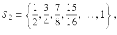
because all points except 1 are isolated, hence removed in the first step. After that, 1 is isolated, so it is removed in the second step. By cramming sets like S 2 into the intervals ![]() and finally adding the point 2, we get a set S 3 for which it takes three steps to remove all points: the first step leaves
and finally adding the point 2, we get a set S 3 for which it takes three steps to remove all points: the first step leaves ![]() , and the second step leaves 2, which is removed at the third step.
, and the second step leaves 2, which is removed at the third step.
It is easy to iterate this idea to obtain a set S n that is emptied only by n removals of isolated points. Then, by suitably compressing the sets ![]() into a convergent sequence of adjacent intervals, we obtain a set S that is not exhausted by
into a convergent sequence of adjacent intervals, we obtain a set S that is not exhausted by ![]() removals of isolated points. However, we can arrange that just one point of S remains after this infinite sequence of removals, so it makes sense to say that S is emptied at the first step after steps
removals of isolated points. However, we can arrange that just one point of S remains after this infinite sequence of removals, so it makes sense to say that S is emptied at the first step after steps ![]() . The first step after
. The first step after ![]() is called step ω, and the ordinal number ω is naturally defined to be the set of all its predecessors, namely
is called step ω, and the ordinal number ω is naturally defined to be the set of all its predecessors, namely
![]()
The successor function ![]() applies to ordinals just as well as it does to natural numbers, so we get another increasing sequence of numbers
applies to ordinals just as well as it does to natural numbers, so we get another increasing sequence of numbers
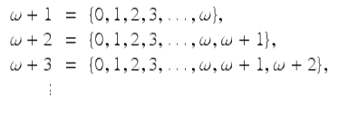
There is likewise a first ordinal number after all of these, namely
![]()
In general, for any set A of ordinal numbers, the set ![]() is an ordinal number. If
is an ordinal number. If ![]() is not a successor, as is the case when A has no greatest member, then
is not a successor, as is the case when A has no greatest member, then ![]() is called a limit ordinal and
is called a limit ordinal and ![]() is the limit of the set A. This powerful limit operation produces ordinals big enough to measure not merely “how long” a process on real numbers can run, but “how long” it takes to construct any set by means of the ZF set construction operations.
is the limit of the set A. This powerful limit operation produces ordinals big enough to measure not merely “how long” a process on real numbers can run, but “how long” it takes to construct any set by means of the ZF set construction operations.
The construction of sets is hitched to the construction of ordinals as follows. If
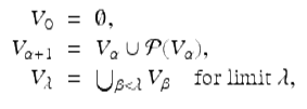
then the subscripts α run through all the ordinal numbers and every set X occurs in some V α . It is actually the same to let ![]() , but the above definition makes it clearer that a member of V α also belongs to all higher Vβ . The least α such that
, but the above definition makes it clearer that a member of V α also belongs to all higher Vβ . The least α such that ![]() (“how long” it takes to construct X) is called the rank of X. In particular, the rank of each ordinal α is α.
(“how long” it takes to construct X) is called the rank of X. In particular, the rank of each ordinal α is α.
7 Large Cardinals
We mentioned in Section 5 that the Infinity axiom is not provable from the other axioms of ZF. It is now worth explaining in more detail why this is so, since similar details occur in showing that certain large cardinal axioms are not provable in ZF.
The first thing to notice is that Infinity does not hold in V ω , the union of the sets ![]() . This is because V 0 = ∅ and
. This is because V 0 = ∅ and ![]() , whence it easily follows by induction that all sets in each V n are finite.
, whence it easily follows by induction that all sets in each V n are finite.
The second thing is that V ω satisfies all the other axioms of ZF. The only ones that are not quite obvious are the set construction axioms, and these hold for the following reasons.
Pairing.
If A, B ∈ V n then ![]() , because all subsets of V n belong to V n+1.
, because all subsets of V n belong to V n+1.
Union.
Suppose X ∈ V n+2, and y ∈ x ∈ X. Then ![]() and y ∈ V n . Thus
and y ∈ V n . Thus ![]() is a subset of V n and hence a member of V n+1.
is a subset of V n and hence a member of V n+1.
Power Set.
Suppose ![]() , so any members of X are in V n . Then each subset of X is a subset of V n , hence a member of V n+1.
, so any members of X are in V n . Then each subset of X is a subset of V n , hence a member of V n+1. ![]() is therefore a subset of V n+1, hence a member of V n+2.
is therefore a subset of V n+1, hence a member of V n+2.
Replacement.
Suppose f is a definable function whose domain is some X ∈ V n and whose values lie in V ω . Since all members of V n are finite, the range of f is finite, hence all of its members lie in some V m . But then the range of f is a member of V m+1.
Thus V ω is a model of all the axioms of ZF except the Infinity axiom. Since the Infinity axiom does not hold in V ω , it cannot be a logical consequence of the other axioms.
Now we are ready to consider a large cardinal axiom; namely, one asserting the existence of an inaccessible V α . V α is called inaccessible if it has ![]() as a member and is closed under the power set and replacement operations. That is, if
as a member and is closed under the power set and replacement operations. That is, if ![]() , then
, then ![]() , and if f is a function whose domain belongs to V α then the range of f also belongs to V α .
, and if f is a function whose domain belongs to V α then the range of f also belongs to V α .
Since V α has ![]() as a member, V α satisfies the Infinity axiom, and it satisfies Power Set and Replacement because of its closure under the power set and replacement operations. The remaining axioms of ZF hold for the same reasons that they hold in V ω (bearing in mind that α must be a limit ordinal for closure under the power set operation). Thus an inaccessible V α satisfies all the axioms of ZF. No inaccessible V α is actually known, however—it is not called “inaccessible” for nothing! This is due to the remarkable fact, essentially noticed by Kuratowski in 1924: if an inaccessible V α exists, then its existence is not provable in ZF.
as a member, V α satisfies the Infinity axiom, and it satisfies Power Set and Replacement because of its closure under the power set and replacement operations. The remaining axioms of ZF hold for the same reasons that they hold in V ω (bearing in mind that α must be a limit ordinal for closure under the power set operation). Thus an inaccessible V α satisfies all the axioms of ZF. No inaccessible V α is actually known, however—it is not called “inaccessible” for nothing! This is due to the remarkable fact, essentially noticed by Kuratowski in 1924: if an inaccessible V α exists, then its existence is not provable in ZF.
The explanation of this fact is quite simple. If an inaccessible V α exists, take the one with smallest possible α (which exists by the Foundation axiom). Then the V β belonging to V α are not inaccessible because β < α. Thus V αsatisfies not only the ZF axioms but also the sentence “There is no inaccessible V α .” This means that the existence of an inaccessible V α is not a logical consequence of ZF.3
8 Measuring Subsets of ![]()
In Section 2 we observed the power of infinite operations (specifically, countable unions) to determine lengths and areas. The example of the parabolic segment dramatically shows how a complicated region can be measured by cutting it into a countable infinity of parts (triangles) whose measure is known. The completeness of ![]() also plays a role, by allowing the formation of infinite sums of measures.
also plays a role, by allowing the formation of infinite sums of measures.
So, given that we need countable unions to determine measures, the question arises: which regions are measurable when we allow countable unions? To make the question as simple and definite as possible, let us confine attention to subsets of the unit interval [0,1], and impose the following conditions on the measure μ.
Measure of an interval.
![]() .
.
Subtractivity.
If S, T are measurable and ![]() , then
, then
![]()
Countable additivity.
If S 1, S 2, S 3, … are disjoint measurable sets, then
![]()
Notice that the measure of an interval implies that ![]() . Subtractivity then implies that [a, b], (a, b], [a, b), and (a, b) all have measure b − a. It also follows from countable additivity that any countable set has measure zero, as we already observed in Section 2.
. Subtractivity then implies that [a, b], (a, b], [a, b), and (a, b) all have measure b − a. It also follows from countable additivity that any countable set has measure zero, as we already observed in Section 2.
Another consequence of subtractivity is that the complement [0, 1] − S of any measurable set S is measurable. It also follows (not so obviously) from countable additivity that the countable union ![]() of not necessarily disjoint measurable sets
of not necessarily disjoint measurable sets ![]() is measurable. Thus the class of measurable sets includes all sets obtainable from open intervals by the operations of complement and countable union. These are called the Borelsets after Émile Borel, who in 1898 outlined essentially the approach to measure I have just described.
is measurable. Thus the class of measurable sets includes all sets obtainable from open intervals by the operations of complement and countable union. These are called the Borelsets after Émile Borel, who in 1898 outlined essentially the approach to measure I have just described.
However, by adding some plausible extra assumptions to ZF (see the next section) we can prove that there are only continuum-many Borel sets, so not all subsets of [0,1] are Borel. Fortunately, there is a natural extension of Borel’s measure concept that covers many more sets (as many as there are subsets of ![]() or [0,1]). This is the concept of Lebesgue measure, introduced by Lebesgue in 1902.
or [0,1]). This is the concept of Lebesgue measure, introduced by Lebesgue in 1902.
Lebesgue assigns measure zero to any subset of a Borel set of measure zero, thereby assigning a measure to any set that differs from a Borel set by a set of measure zero. Under the same assumptions that support the theory of Borel sets it then becomes possible that all subsets of [0,1] are Lebesgue measurable. “Possible” does not mean provable, but consistent, in the following sense.
If ZF+“an inaccessible V α exists” is consistent,
then so is ZF+“all subsets of [0,1] are Lebesgue measurable.”
This result was proved by Solovay in 1965, and in 1984 Shelah showed that the assumption of inaccessibility cannot be dropped. So, a problem about ![]() is settled only by assuming the existence of a set large enough to model the whole of set theory. Somehow, a question about
is settled only by assuming the existence of a set large enough to model the whole of set theory. Somehow, a question about ![]() “blows up” to a question about the whole universe.
“blows up” to a question about the whole universe.
This is not an isolated example, as we will see in the next section.
9 Nonmeasurable Sets and the Axiom of Choice
Since it is consistent with ZF for all subsets of [0,1] to be measurable, only a new axiom can give us a nonmeasurable set. Do we want such an axiom? The general consensus is that we do, and in fact such an axiom has been around for over 100 years: the axiom of choice (AC for short).
In the late 19th century certain forms of AC were assumed, or used unconsciously, to prove results such as the countability of a countable union of countable sets.4 But AC escaped attention until 1904, when Zermelo used it to prove the surprising theorem that every set can be well-ordered (that is, linearly ordered in such a way that every subset has a least element). AC states that every set X of nonempty sets x has a choice function: a function f such that f(x) ∈ x for each x ∈ X. The converse theorem, that well-ordering implies AC, is almost obvious because f(x) can be defined as the least member of x in a suitable well-ordering.
Now well-ordering obviously simplifies the world of sets—for example, it means that every set has the same cardinality as an ordinal—so one would have expected AC to be welcome. In fact, it received a hostile reception from Borel, Lebesgue, and many other eminent mathematicians. They objected to the apparent undefinability of the choice function f, which is indeed a mystery in the important case where the sets x are nonempty subsets of ![]() .
.
Also, AC had some unwelcome consequences, such as nonmeasurable subsets of [0,1]. This was proved by Vitali in 1905.
To explain Vitali’s proof it is convenient to imagine [0,1] made into a circle of circumference 1 by joining its two ends. Then we partition [0,1] into equivalence classes, where a and b declared to be equivalent if b − a is rational. Thus the rational numbers in [0,1] form one equivalence class R. Every other class is the translate ![]() of R through an irrational distance
of R through an irrational distance ![]() . (This is where it is convenient to view [0,1] as a circle: translation through distance
. (This is where it is convenient to view [0,1] as a circle: translation through distance ![]() means moving each point around the circumference through distance
means moving each point around the circumference through distance ![]() .)
.)
Now AC says that we can form a set S with exactly one member from each distinct equivalence class ![]() . It follows that the translate S + r of S through a rational distance r ≠ 0 in [0,1] is disjoint from S, because the representative of each equivalence class is translated to a different representative. Moreover, as r runs through all the nonzero rationals in [0,1], the points in S + r run through all representatives of all equivalence classes.
. It follows that the translate S + r of S through a rational distance r ≠ 0 in [0,1] is disjoint from S, because the representative of each equivalence class is translated to a different representative. Moreover, as r runs through all the nonzero rationals in [0,1], the points in S + r run through all representatives of all equivalence classes.
Thus the countably many disjoint sets S + r fill the circle of circumference 1. Finally, notice that if S is measurable then all the sets S + r have the same measure, because Lebesgue measure is translation-invariant (due to the fact that translates of any interval have the same measure). But now there are only two possibilities: μ(S) = 0 or μ(S) > 0. By countable additivity, the first implies that μ([0, 1]) = 0 and the second implies that ![]() . Both of these conclusions are false, so S is not measurable.
. Both of these conclusions are false, so S is not measurable.
This is a painful predicament. To have measure theory at all, we need some form of AC—in particular we need a countable union of countable sets to be countable—but AC tells us that we cannot measure all subsets of [0,1]. Solovay’s model offers a way out of this predicament, because it satisfies a weaker axiom of choice, called dependent choice, which is strong enough to support measure theory. (In particular, dependent choice implies that a countable union of countable sets is countable.) However, mathematicians today are hooked on AC. Algebraists like it as much as set theorists do, because the equivalents of AC include some desirable theorems of algebra. Among them are the existence of a basis for any vector space, and the existence of a maximal ideal for any nontrivial ring.
Thus, in the universe now favored by most mathematicians, there are nonmeasurable sets of real numbers. The question up for negotiation is: how complex are the nonmeasurable sets? The answer to this question depends on large cardinals, and in fact on cardinals much larger than the inaccessible required for Solovay’s model.
We already know that the measurable sets include all Borel sets. The simplest class that includes non-Borel sets is that class called the analytic, or ![]() , sets, which are the projections of Borel sets in
, sets, which are the projections of Borel sets in ![]() onto
onto ![]() . They, and their complements the
. They, and their complements the ![]() sets, were shown to be measurable by Luzin in 1917. These two classes form the first level of the so-called projective sets, which are obtained from Borel sets in
sets, were shown to be measurable by Luzin in 1917. These two classes form the first level of the so-called projective sets, which are obtained from Borel sets in ![]() by alternate operations of projection and complementation. In 1925, Luzin declared prophetically that “one does not know and one will never know” whether all projective sets are measurable. Maybe he was right.
by alternate operations of projection and complementation. In 1925, Luzin declared prophetically that “one does not know and one will never know” whether all projective sets are measurable. Maybe he was right.
In 1938 Gödel showed that it is consistent with ZF+AC to have nonmeasurable sets at the second level of the projective hierarchy, ![]() . This result is a corollary of his momentous proof that:
. This result is a corollary of his momentous proof that:
![]()
Gödel proved this result by defining a class L of what he called constructible sets, each of which has a definition in a language obtained from the ZF language by adding symbols for all the ordinals. The definitions of this language can be well-ordered, so L satisfies the well-ordering theorem and hence AC. Moreover, L satisfies all the axioms of ZF, because there are enough constructible sets to satisfy the set construction axioms. It turns out that the well-ordering of constructible real numbers is in ![]() , and this gives a nonmeasurable set at the same level.
, and this gives a nonmeasurable set at the same level.
Thus the assumption that all sets are constructible—an assumption that the universe is in some sense “small”—gives nonmeasurable sets that are as simple as they can be, in terms of the projective hierarchy. At the other extreme, it is possible that all projective sets are measurable, under the assumption that sufficiently large cardinals exist. This was proved in 1985 by Martin and Steel, and the necessary large cardinals are called Woodin cardinals. They are considerably larger than the inaccessible cardinal required for Solovay’s model, so their existence is even more problematic.
Once again, a question about the real numbers “blows up” to a question about the size of the whole universe of sets.
10 Summing Up
The aim of this chapter has been to give a glimpse of our ignorance about ![]() and to emphasize that some questions about
and to emphasize that some questions about ![]() call for further axioms about the whole universe of sets. Readers with some knowledge of mathematical logic will know that the same is true of
call for further axioms about the whole universe of sets. Readers with some knowledge of mathematical logic will know that the same is true of ![]() because of Gödel’s incompleteness theorem. However, there seems to be a difference between
because of Gödel’s incompleteness theorem. However, there seems to be a difference between ![]() and
and ![]() . The only known questions about
. The only known questions about ![]() that depend on large cardinals are ones concocted by logicians; in the case of
that depend on large cardinals are ones concocted by logicians; in the case of ![]() , the questions that depend on large cardinals include some that arose naturally, before large cardinals had even been imagined.
, the questions that depend on large cardinals include some that arose naturally, before large cardinals had even been imagined.
Thus ![]() , much more so than
, much more so than ![]() , is the true gateway to infinity.
, is the true gateway to infinity. ![]() is the largely avoidable “potential” infinity of the Greeks;
is the largely avoidable “potential” infinity of the Greeks; ![]() is an actual infinity forced upon us by the apparent continuity of the natural world. If we are committed to understanding
is an actual infinity forced upon us by the apparent continuity of the natural world. If we are committed to understanding ![]() , then we are committed to understanding the whole universe of sets.
, then we are committed to understanding the whole universe of sets.
Yet, admittedly, it is a mystery how we can understand anything about ![]() . What are we thinking when we think about
. What are we thinking when we think about ![]() ?
?
11 Further Reading
There is a dearth of literature for students, or even the ordinary mathematician, about ![]() and its relations to set theory and logic. I attempted to remedy this situation with a semi-popular book, Roads to Infinity (AK Peters 2010) and an undergraduate text The Real Numbers (Springer 2013).
and its relations to set theory and logic. I attempted to remedy this situation with a semi-popular book, Roads to Infinity (AK Peters 2010) and an undergraduate text The Real Numbers (Springer 2013).
Beyond that, you will have to consult quite serious set theory books for results such as Solovay’s model in which all sets of reals are Lebesgue measurable. The standard one is Jech’s Set Theory (3rd edition, Springer 2003). A more recent, and less bulky, book that also covers Solovay’s model and Woodin cardinals is Schindler’s Set Theory (Springer 2014). Finally, for the general theory of large cardinals, with many interesting historical remarks, see Kanamori The Higher Infinite (Springer 2003).
Footnotes
1
The ancient Greeks had a much more complicated theory of measure, in which the measure of a rectangle is the rectangle itself, and two rectangles have the same measure only if one can be cut up and reassembled to form the other.
2
This argument was discovered by Harnack in 1885, but he was confused about what it meant. It seemed to him that covering all the rationals in [0,1] by intervals would cover all points in [0,1], so an interval of length 1 could be covered intervals of total length ![]() . Fortunately for measure theory, this is impossible, because of the Heine-Borel theorem that if an infinite collection of open intervals covers [0,1] you can extract a finite subcollection that also covers [0,1]. By unifying any overlapping intervals in the finite covering you get a covering of [0,1] by finitely many open disjoint intervals of total length
. Fortunately for measure theory, this is impossible, because of the Heine-Borel theorem that if an infinite collection of open intervals covers [0,1] you can extract a finite subcollection that also covers [0,1]. By unifying any overlapping intervals in the finite covering you get a covering of [0,1] by finitely many open disjoint intervals of total length ![]() , which is clearly impossible.
, which is clearly impossible.
It was to deal with precisely this problem that Borel in 1898 introduced the Heine-Borel theorem. He called it “the first fundamental theorem of measure theory.”
3
Unless of course ZF is inconsistent, in which case any sentence is a logical consequence of ZF. Thus whenever we show that something is not provable in ZF we are implicitly assuming that ZF is consistent. This is an unavoidable assumption because the consistency of ZF cannot be proved from the ZF axioms. The above argument shows the futility of one approach to proving consistency—by finding a V α that satisfies the ZF axioms—and in fact any approach must fail by Gödel’s famous second incompleteness theorem.
4
Not only is this result unprovable without some form of AC, it is even consistent with ZF for ![]() to be a countable union of countable sets. This amazing result was proved by Feferman and Levy in 1963. It implies that every subset of
to be a countable union of countable sets. This amazing result was proved by Feferman and Levy in 1963. It implies that every subset of ![]() is a Borel set, but at the same time wrecks the theory of measure, because countable sets have measure zero and a countable union of measure zero sets is also supposed to have zero measure.
is a Borel set, but at the same time wrecks the theory of measure, because countable sets have measure zero and a countable union of measure zero sets is also supposed to have zero measure.
Thus for both the theory of Borel sets and for measure theory we want a countable union of countable sets to be countable. One axiom that implies this is the so-called countable axiom of choice, whose statement is the same as AC but with the extra condition that X is countable.