Pre-Calculus For Dummies, 2nd Edition (2012)
Part III. Analytic Geometry and System Solving
Chapter 12. Slicing Cones or Measuring the Path of a Comet - with Confidence
In This Chapter
![]() Spinning around with circles
Spinning around with circles
![]() Dissecting the parts and graphs of parabolas
Dissecting the parts and graphs of parabolas
![]() Exploring the ellipse
Exploring the ellipse
![]() Boxing around with hyperbolas
Boxing around with hyperbolas
![]() Writing and graphing conics in two distinct forms
Writing and graphing conics in two distinct forms
Astronomers have been looking out into space for a very long time — longer than you’ve been staring at the ceiling during class. Some of the things that are happening out there are mysteries; others have shown their true colors to curious observers. One phenomenon that astronomers have discovered and proven is the movement of bodies in space. They know that the paths of objects moving in space are shaped like one of four conic sections (shapes made from cones): the circle, the parabola, the ellipse, or the hyperbola. Conic sections have evolved into popular ways to describe motion, light, and other natural occurrences in the physical world.
In astronomical terms, an ellipse, for example, describes the path of a planet around the sun. A comet may travel so close to a planet’s gravity that its path is affected and it gets swung back out into the galaxy. If you were to attach a gigantic pen to the comet, its path would trace out one huge parabola. The movement of objects as they are affected by gravity can often be described using conic sections. For example, you can describe the movement of a ball being thrown up into the air using a conic section. As you can see, the conic sections you study in pre-calculus have plenty of applications — especially for rocket science!
Conic sections are so named because they’re made from two right circular cones (imagine two sugar cones from your favorite ice-cream store). Basically, you see two right circular cones, touching pointy end to pointy end (the pointy end of a cone is called the element). The conic sections are formed by the intersection of a plane and the ice-cream cones. When you slice through the cones with a plane, the intersection of that plane with the cones yields a variety of different curves. The plane is completely arbitrary, and where it cuts the cone and at what angle are what give you all the different conic sections that we discuss in this chapter.
In this chapter, we break down each of the conic sections, front to back. We discuss the similarities and the differences between the four conic sections and their applications in pre-calculus. We also graph each section and look at its properties. Conic sections are the final frontier when it comes to graphing in mathematics, so sit back, relax, and enjoy the ride!
Cone to Cone: Identifying the Four Conic Sections
Each conic section has its own standard form of an equation with x- and y-variables that you can graph on the coordinate plane. You can write the equation of a conic section if you are given key points on the graph, or you can graph the conic section from the equation. You can alter the shape of each of these graphs in various ways, but the general graph shapes still remain true to the type of curve that they are.
Being able to identify which conic section is which by just the equation is important because sometimes that’s all you’re given (you won’t always be told what type of curve you’re graphing). Certain key points are common to all conics (vertices, foci, and axes, to name a few), so you start by plotting these key points and then identifying what kind of curve they form.
In picture (Graph form)
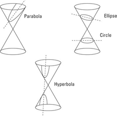
The whole point of this chapter is to be able to graph conic sections accurately with all the necessary information. Figure 12-1 illustrates how a plane intersects the cones to create the conic sections, and the following list explains the figure:
![]() Circle: A circle is the set of all points that are a given distance (the radius, r) from a given point (the center). To get a circle from the right cones, the plane slice occurs parallel to the base of either cone but doesn’t slice through the element of the cones.
Circle: A circle is the set of all points that are a given distance (the radius, r) from a given point (the center). To get a circle from the right cones, the plane slice occurs parallel to the base of either cone but doesn’t slice through the element of the cones.
![]() Parabola: A parabola is a curve in which every point is equidistant from one point (the focus) and a line (the directrix). It looks a lot like the letter U, although it may be upside down or sideways. To form a parabola, the plane slices through parallel to the side of the cones (any side works, but the bottom and top are forbidden).
Parabola: A parabola is a curve in which every point is equidistant from one point (the focus) and a line (the directrix). It looks a lot like the letter U, although it may be upside down or sideways. To form a parabola, the plane slices through parallel to the side of the cones (any side works, but the bottom and top are forbidden).
![]() Ellipse: An ellipse is the set of all points where the sum of the distances from two points (the foci) is constant. You may be more familiar with another term for ellipse, oval. In order to get an ellipse from the two right cones, the plane must cut through one cone, not parallel to the base, and not through the element.
Ellipse: An ellipse is the set of all points where the sum of the distances from two points (the foci) is constant. You may be more familiar with another term for ellipse, oval. In order to get an ellipse from the two right cones, the plane must cut through one cone, not parallel to the base, and not through the element.
![]() Hyperbola: A hyperbola is the set of points where the difference of the distances between two points is constant. The shape of the hyperbola is difficult to describe without a picture, but it looks visually like two parabolas (although they’re very different mathematically) mirroring one another with some space between the vertices. To get a hyperbola, the slice cuts the cones perpendicular to their bases (straight up and down) but not through the element.
Hyperbola: A hyperbola is the set of points where the difference of the distances between two points is constant. The shape of the hyperbola is difficult to describe without a picture, but it looks visually like two parabolas (although they’re very different mathematically) mirroring one another with some space between the vertices. To get a hyperbola, the slice cuts the cones perpendicular to their bases (straight up and down) but not through the element.
Figure 12-1:Cutting cones with a plane to get conic sections.
 Most of the time, sketching a conic is not enough. Each conic section has its own set of information that you usually have to give to supplement the graph. You have to indicate where the center, vertices, major and minor axes, and foci are located. Oftentimes, this information is more important than the graph itself. Besides, knowing all this valuable info helps you sketch the graph more accurately than you could without it.
In print (Equation form)
The equations of conic sections are very important because they not only tell you which conic section you should be graphing but also tell you what the graph should look like. The appearance of each conic section has trends based on the values of the constants in the equation. Usually these constants are referred to as a, b, h, v, f, and d. Not every conic has all these constants, but conics that do have them are affected in the same way by changes in the same constant. Conic sections can come in all different shapes and sizes: big, small, fat, skinny, vertical, horizontal, and more. The constants listed above are the culprits of these changes.
 An equation has to have x2 and/or y2 to create a conic. If neither x nor y is squared, then the equation is of a line (not considered a conic section for our purposes in this book). None of the variables of a conic section may be raised to any power higher than two.
As briefly mentioned, certain characteristics are unique to each type of conic and hint to you which of the conic sections you’re graphing. In order to recognize these characteristics the way we wrote them, the x2 term and the y2term must be on the same side of the equal sign. If they are, then these characteristics are as follows:
![]() Circle: When x and y are both squared and the coefficients on them are the same — including the sign.
Circle: When x and y are both squared and the coefficients on them are the same — including the sign.
For example, take a look at 3x2 – 12x + 3y2 = 2. Notice that the x2 and y2 have the same coefficient (positive 3). That info is all you need to recognize that you’re working with a circle.
![]() Parabola: When either x or y is squared — not both.
Parabola: When either x or y is squared — not both.
The equations y = x2 – 4 and x = 2y2 – 3y + 10 are both parabolas. In the first equation, you see an x2 but no y2, and in the second equation, you see a y2 but no x2. Nothing else matters — sign and coefficients change the physical appearance of the parabola (which way it opens or how fat it is) but don’t change the fact that it’s a parabola.
![]() Ellipse: When x and y are both squared and the coefficients are positive but different.
Ellipse: When x and y are both squared and the coefficients are positive but different.
The equation 3x2 – 9x + 2y2 + 10y – 6 = 0 is one example of an ellipse. The coefficients on x2 and y2 are different, but both are positive.
![]() Hyperbola: When x and y are both squared and exactly one of the coefficients is negative (coefficients may be the same or different).
Hyperbola: When x and y are both squared and exactly one of the coefficients is negative (coefficients may be the same or different).
The equation 4y2 – 10y – 3x2 = 12 is an example of a hyperbola. This time, the coefficients on x2 and y2 are different, but one of them is negative, which is a requirement to get the graph of a hyperbola.
 The equations for the four conic sections look very similar to one another, with subtle differences (a plus sign instead of a minus sign, for instance, gives you an entirely different type of conic section). If you get the forms of equations mixed up, you’ll end up graphing the wrong shape, so be forewarned!
Going Round and Round: Graphing Circles
Circles are simple to work with in pre-calculus. A circle has one center, one radius, and a whole lot of points. In this section, we show you how to graph circles on the coordinate plane and figure out from both the graph and the circle’s equation where the center lies and what the radius is.
The first thing you need to know in order to graph the equation of a circle is where on a plane the center is located. The equation of a circle appears as (x – h)2 + (y – v)2 = r2. We call this form the center-radius form (or standard form) because it gives you both pieces of information at the same time. The h and v represent the center of the circle at point (h, v), and r names the radius. Specifically, h represents the horizontal displacement — how far to the left or to the right of the y-axis the center of the circle is. The variable v represents the vertical displacement — how far above or below the x-axis the center falls. From the center, you can count from the center r units (the radius) horizontally in both directions and vertically in both directions to get four different points, all equidistant from the center. Connect these four points with the best curve that you can sketch to get the graph of the circle.
Graphing circles at the origin
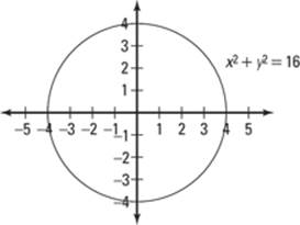
The simplest circle to graph has its center at the origin (0, 0). Because both h and v are zero, they can disappear and you can simplify the standard circle equation to look like x2 + y2 = r2. For instance, to graph the circle x2 + y2 = 16, follow these steps:
1. Realize that the circle is centered at the origin (no h and v) and place this point there.
2. Calculate the radius by solving for r.
Set r2 = 16. In this case, you get r = 4.
3. Plot the radius points on the coordinate plane.
You count out 4 in every direction from the center (0, 0): left, right, up, and down.
4. Connect the dots to graph the circle using a smooth, round curve.
Figure 12-2 shows this circle on the plane.
Figure 12-2:Graphing a circle centered at the origin.
Graphing circles away from the origin
Graphing a circle anywhere on the coordinate plane is pretty easy when its equation appears in center-radius form. All you do is plot the center of the circle at (h, k), count out from the center r units in the four directions (up, down, left, right), and connect those four points with a circle. Unfortunately, although graphing circles at the origin is easiest, very few graphs are as straightforward and simple as those. In pre-calc, you work with transforming graphs of all different shapes and sizes (nothing new to you, right?). Fortunately, these graphs all follow the same pattern for horizontal and vertical shifts, so you don’t have to remember many rules.
Don’t forget to switch the sign of the h and v from inside the parentheses in the equation. This step is necessary because the h and v are inside the grouping symbols, which means that the shift happens opposite from what you would think (see Chapter 3 for more information on shifting graphs).
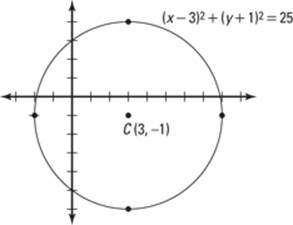
For example, follow these steps to graph the equation (x – 3)2 + (y + 1)2 = 25:
1. Locate the center of the circle from the equation (h, v).
(x – 3)2 means that the x-coordinate of the center is positive 3.
(y + 1)2 means that the y-coordinate of the center is negative 1.
Place the center of the circle at (3, –1).
2. Calculate the radius by solving for r.
Set r2 = 25 and square root both sides to get r = 5.
3. Plot the radius points on the coordinate plane.
Count 5 units up, down, left, and right from the center at (3, –1). This step gives you points at (8, –1), (–2, –1), (3, –6), and (3, 4).
4. Connect the dots to the graph of the circle with a round, smooth curve.
See Figure 12-3 for a visual representation of this circle.
Figure 12-3:Graphing a circle not centered at the origin.
 Some books use h and k to represent the horizontal and vertical displacement of circles. However, we refer to the shifts as h for the horizontal shift and v for the vertical shift. We don’t know why other people chose hand k, but we think h and v are much easier to remember!
Sometimes the equation is in center-radius form (and then graphing is a piece of cake), and sometimes you have to manipulate the equation a bit to get it into a form that’s easy for you to work with. When a circle doesn’t appear in center-radius form, you have to complete the square in order to find the center. (We talk about this process in Chapter 4, so if you’re unfamiliar with it, head back there for a refresher.)
Riding the Ups and Downs with Parabolas
Although parabolas look like simple U-shaped curves, very complicated variables make them look the way they do. Because they involve squaring one value (and one value only), they become a mirror image over the axis of symmetry, just like the quadratic functions from Chapter 3. Because a positive number squared is positive, and the opposite of that number (a negative one) is also positive, you get a U-shaped graph.
The parabolas we discuss in Chapter 3 are all quadratic functions, which means that they passed the vertical-line test. The purpose of parabolas in this chapter, however, is to discuss them not as functions but rather as conic sections. What’s the difference, you ask? Quadratic functions must fit the definition of a function, whereas if we discuss parabolas as conic sections, they can be vertical (like the functions) or horizontal (like a sideways U, which doesn’t fit the definition of passing the vertical-line test).
In this section, we introduce you to different parabolas that you encounter on your journey through conic sections.
Labeling the parts
Each of the different parabolas in this section has the same general shape; however, the width of the parabolas, their location on the coordinate plane, and which direction they open can vary greatly from one another.
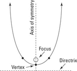
One thing that’s true of all parabolas is their symmetry, meaning that you can fold a parabola in half over itself. The line that divides a parabola in half is called the axis of symmetry. The focus is a point inside (not on) the parabola that lies on the axis of symmetry, and the directrix is a line that runs outside the parabola perpendicular to the axis of symmetry. The vertex of the parabola is exactly halfway between the focus and the directrix. Recall from geometry that the distance from any line to a point not on that line is a line segment from the point perpendicular to the line. Therefore, the parabola is formed by all the points equidistant from the focus and the directrix. The distance between the vertex and the focus, then, dictates how skinny or how fat the parabola is.
The first thing you must find in order to graph a parabola is where the vertex is located. From there, you can find out whether it should be up and down (a vertical parabola) or sideways (a horizontal parabola). The coefficients of the parabola also tell you which way the parabola opens (toward the positive numbers or the negative numbers).
If you’re graphing a vertical parabola, then the vertex is also the maximum or the minimum value of the curve. Calculating the maximum and minimum values has tons of real-world applications for you to dive into. Bigger is usually better, and maximum area is no different. Parabolas are very useful in telling you the maximum (or sometimes minimum) area for rectangles. For example, if you’re building a dog run with a preset amount of fencing, you can use parabolas to find the dimensions of the dog run that would yield the maximum area for your dog to run.
Understanding the characteristics of a standard parabola
The squaring of the variables in the equation of the parabola determines where it opens:
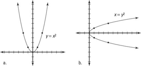
![]() When the x is squared and y is not: In this case, the axis of symmetry is vertical and the parabola opens up or down. For instance, y = x2 is a vertical parabola; its graph is shown in Figure 12-4a.
When the x is squared and y is not: In this case, the axis of symmetry is vertical and the parabola opens up or down. For instance, y = x2 is a vertical parabola; its graph is shown in Figure 12-4a.
![]() When y is squared and x is not: In this case, the axis of symmetry is horizontal and the parabola opens left or right. For example, x = y2 is a horizontal parabola; it’s shown in Figure 12-4b.
When y is squared and x is not: In this case, the axis of symmetry is horizontal and the parabola opens left or right. For example, x = y2 is a horizontal parabola; it’s shown in Figure 12-4b.
Both of these parabolas have the vertex located at the origin.
Be aware of negative coefficients in parabolas. If the parabola is vertical, a negative coefficient makes the parabola open downward. If the parabola is horizontal, a negative coefficient makes the parabola open to the left.
Figure 12-4: A vertical and horizontal parabola based at the origin.
Plotting the variations: Parabolas all over the plane (Not at the origin)
Just like with circles, the vertex of the parabola isn’t always at the origin. You need to be comfortable with shifting parabolas around the coordinate plane too. Certain motions, especially the motion of falling objects, move in a parabolic shape with respect to time. For example, the height of a ball launched up in the air at time t can be described by the equation h(t)= –16t2 + 32t. Finding the vertex of this equation tells you the maximum height of the ball and also when the ball reached that height. Finding the x-intercepts also tells you when the ball will hit the ground again.
A vertical parabola written in the form y = a(x – h)2 + v gives you the following information:
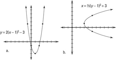
![]() A vertical transformation (designated by the variable a): For instance, for y = 2(x – 1)2 – 3, every point is stretched vertically by a factor of 2 (see Figure 12-5a for the graph). Therefore, every time you plot a point on the graph, the original height of y = x2 is multiplied by 2.
A vertical transformation (designated by the variable a): For instance, for y = 2(x – 1)2 – 3, every point is stretched vertically by a factor of 2 (see Figure 12-5a for the graph). Therefore, every time you plot a point on the graph, the original height of y = x2 is multiplied by 2.
![]() The horizontal shift of the graph (designated by the variable h): In this example, the vertex is shifted to the right of the origin 1 unit (–h; don’t forget to switch the sign inside the parentheses).
The horizontal shift of the graph (designated by the variable h): In this example, the vertex is shifted to the right of the origin 1 unit (–h; don’t forget to switch the sign inside the parentheses).
![]() The vertical shift of the graph (designated by the variable v): In this example, the vertex is shifted down 3 (+ v).
The vertical shift of the graph (designated by the variable v): In this example, the vertex is shifted down 3 (+ v).
 All vertical parabolas with a vertical transformation of 1 move in the following pattern after you graph the vertex:
1. Right 1, up 12
2. Right 2, up 22
3. Right 3, up 32
This pattern continues. Usually, just a couple of points give you a good graph. You plot the same points on the other side of the vertex to create the mirror image over the axis of symmetry.
The transformations of horizontal parabolas on the coordinate plane are different from the transformations of vertical parabolas, because instead of moving right 1, up 12, right 2, up 22, right 3, up 32, and so on, the parabola is sideways. Therefore, the movement of all horizontal parabolas with a horizontal transformation of one goes
1. Up 1, right 12
2. Up 2, right 22
3. Up 3, right 32
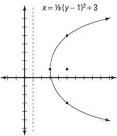
A horizontal parabola appears in the form x = a(y – v)2 + h. In these parabolas, the vertical shift comes with the y variable inside the parentheses (– v), and the
horizontal shift is outside the parentheses (+h). For instance, ![]() has the following characteristics:
has the following characteristics:
It has a vertical transformation of 1/2 at every point.
The vertex is moved up 1 (you switch the sign because it’s inside the parentheses).
The vertex is moved right 3.
You can see this parabola’s graph in Figure 12-5b.
Figure 12-5:Graphing a transformed horizontal parabola.
Finding the vertex, axis of symmetry, focus, and directrix
In order to graph a parabola correctly, you need to note whether the parabola is horizontal or vertical, because although the variables and constants in the equations for both curves serve the same purpose, their effect on the graphs in the end is slightly different. Adding a constant inside the parentheses of the vertical parabola moves the entire thing horizontally, whereas adding a constant inside the parentheses of a horizontal parabola moves it vertically (see the preceding section for more info). You want to note these differences before you start graphing so that you don’t accidentally move your graph in the wrong direction. In the following sections, we show you how to find all this information for both vertical and horizontal parabolas.
Finding points of a vertical parabola
A vertical parabola has its axis of symmetry at x = h, and the vertex is (h, v). With this information, you can find the following parts of the parabola:
![]() Focus: The distance from the vertex to the focus is
Focus: The distance from the vertex to the focus is ![]() , where a can
, where a can
be found in the equation of the parabola (it is the scalar in front of the
parentheses).The focus, as a point, is (h, ![]() ); it should be directly
); it should be directly
above or directly below the vertex. It always appears inside the parabola.
![]() Directrix: The equation of the directrix is
Directrix: The equation of the directrix is ![]() . It is the same
. It is the same
distance from the vertex along the axis of symmetry as the focus, in the opposite direction. The directrix appears outside the parabola and is perpendicular to the axis of symmetry. Because the axis of symmetry is vertical, the directrix is a horizontal line; thus, it has an equation of the
form y = a constant, which is ![]() .
.
Figure 12-6 is something we refer to as the “martini” of parabolas. The graph looks like a martini glass: The axis of symmetry is the glass stem, the directrix is the base of the glass, and the focus is the olive. You need all those parts to make a good martini and a parabola.
Figure 12-6: All the parts of a vertical parabola: shaken, not stirred.
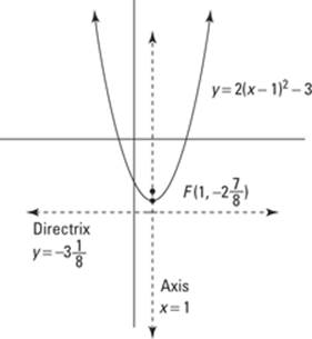
For example, the equation y = 2(x – 1)2 – 3 has its vertex at (1, –3). This means that a = 2, h = 1, and v = –3. With this information, you can identify all the parts of a parabola (axis of symmetry, focus, and directrix) as points or equations:
1. Find the axis of symmetry.
The axis of symmetry is at x = h, which means that x = 1.
2. Determine the focal distance and write the focus as a point.
You can find the focal distance by using the formula ![]() . Because a = 2,
. Because a = 2,
the focal distance for this parabola is ![]() . With this distance, you can
. With this distance, you can
write the focus as the point (h, ![]() ), or (1,
), or (1, ![]() ).
).
3. Find the directrix.
You can use the equation of the directrix: ![]() , or
, or ![]() .
.
4. Graph the parabola and label all its parts.
You can see the graph, with all its parts, in Figure 12-7. We recommend always plotting at least two other points besides the vertex so that you can show that your vertical transformation is correct. Because the vertical transformation in this equation is a factor of 2, the two points on both sides of the vertex are stretched by a factor of 2. So from the vertex, you plot a point that is to the right 1 and up 2 (instead of up 1). Then you can draw the same point on the other side of the axis of symmetry; the two other points on the graph are at (2, –1) and (0, –1).
Figure 12-7:Finding all the parts of the parabola y = 2(x– 1)2 – 3.
Finding points of a horizontal parabola
A horizontal parabola features its own equations to find its parts; these equations are just a bit different from those of a vertical parabola. The distance to the focus and directrix from the vertex in this case is horizontal, because they
move along the axis of symmetry, which is a horizontal line. So ![]() is added to and subtracted from h. Here’s the breakdown:
is added to and subtracted from h. Here’s the breakdown:
![]() The axis of symmetry is at y = v, and the vertex is still at (h, v).
The axis of symmetry is at y = v, and the vertex is still at (h, v).
![]() The focus is directly to the left or right of the vertex, at the point
The focus is directly to the left or right of the vertex, at the point
(![]() , v).
, v).
![]() The directrix is the same distance from the vertex as the focus in the
The directrix is the same distance from the vertex as the focus in the
opposite direction, at ![]() .
.
For example, work with the equation ![]() :
:
1. Find the axis of symmetry.
The vertex of this parabola is (3, 1). The axis of symmetry is at y = v, so for this example, it is at y = 1.
2. Determine the focal distance and write this as a point.
For the equation above, ![]() , and so the focal distance is 2. Add this
, and so the focal distance is 2. Add this
value to h to find the focus: (3 + 2, 1) or (5, 1).
3. Find the directrix.
Subtract the focal distance from Step 2 from h to find the equation of the directrix. Because this parabola is horizontal and the axis of symmetry is horizontal, the directrix is vertical. The equation of the directrix is x = 3 – 2 or x = 1.
4. Graph the parabola and label its parts.
Figure 12-8 shows you the graph and has all of the parts labeled for you.
Figure 12-8:The graph of a horizontal parabola.
The focus lies inside the parabola, and the directrix is a vertical line 2 units to the left from the vertex.
Identifying the min and max on vertical parabolas
Vertical parabolas give an important piece of information: When the parabola opens up, the vertex is the lowest point on the graph — called the minimum. When the parabola opens down, the vertex is the highest point on the graph — called the maximum. Only vertical parabolas can have minimum or maximum values, because horizontal parabolas have no limit on how high or how low they can go. Finding the maximum of a parabola can tell you the maximum height of a ball thrown into the air, the maximum area of a rectangle, the maximum or minimum value of a company’s profit, and so on.
For example, say that a problem asks you to find two numbers whose sum is 10 and whose product is a maximum. You can identify two different equations hidden in this one sentence:
x + y = 10
xy = MAX
If you’re like us, you don’t like to mix variables when you don’t have to, so we suggest that you solve one equation for one variable to substitute into the other one. This process is easiest if you solve the equation that doesn’t include min or max at all. So if x + y = 10, you can say y = 10 – x. You can plug this value into the other equation to get the following:
(10 – x)x = MAX
If you distribute the x on the outside, you get 10x – x2 = MAX. This result is a quadratic equation for which you need to find the vertex by completing the square (which puts the equation into the form you’re used to seeing that identifies the vertex). Finding the vertex by completing the square gives you the maximum value. To do that, follow these steps:
1. Rearrange the terms in descending order.
This step gives you –x2 + 10x = MAX.
2. Factor out the leading term.
You now have –1(x2 – 10x) = MAX.
3. Complete the square (see Chapter 4 for a reference).
This step expands the equation to –1(x2 – 10x + 25) = MAX – 25. Notice that –1 in front of the parentheses turned the 25 into –25, which is why you must add –25 to the right side as well.
4. Factor the information inside the parentheses.
You go down to –1(x – 5)2 = MAX – 25.
5. Move the constant to the other side of the equation.
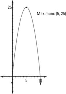
You end up with –1(x – 5)2 + 25 = MAX.
The vertex of the parabola is (5, 25) (see the earlier section “Plotting the variations: Parabolas all over the plane (Not at the origin)”). Therefore, the number you’re looking for (x) is 5, and the maximum product is 25. You can plug 5 in for x to get y in either equation: 5 + y = 10, or y = 5.
Figure 12-9 shows the graph of the maximum function to illustrate that the vertex, in this case, is the maximum point.
By the way, a graphing calculator can easily find the vertex for this type of question. Even in the table form, you can see from the symmetry of the parabola that the vertex is the highest (or the lowest) point.
Figure 12-9:Graphing a parabola to find a maximum value from a word problem.
The Fat and the Skinny on the Ellipse (A Fancy Word for Oval)
An ellipse is a set of points on plane, creating an oval, curved shape such that the sum of the distances from any point on the curve to two fixed points (the foci) is a constant (always the same). An ellipse is basically a circle that has been squished either horizontally or vertically.
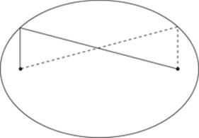
Are you more of a visual learner? Here’s how you can picture an ellipse: Take a piece of paper and pin it to a corkboard with two pins. Tie a piece of string around the two pins with a little bit of slack. Using a pencil, pull the string taut and then trace a shape around the pins — keeping the string taut the entire time. The shape you draw with this technique is an ellipse. The sums of the distances to the pins, then, is the string. The length of the string is always the same in a given ellipse, and different lengths of string give you different ellipses.
This definition that refers to the sums of distances can give even the best of mathematicians a headache because the idea of adding distances together can be difficult to visualize. Figure 12-10 shows you what we mean. The total distance on the solid line is equal to the total distance on the dotted line.
Figure 12-10: A ellipse marked with its foci.
Labeling ellipses and expressing them with algebra
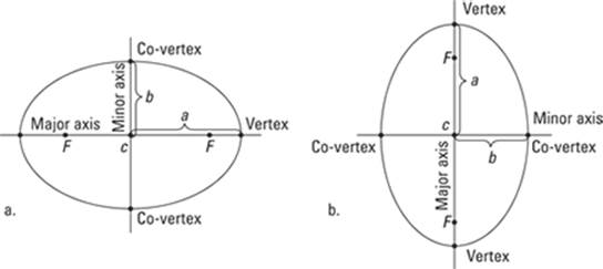
Graphically speaking, you must know two different types of ellipses: horizontal and vertical. A horizontal ellipse is short and fat; a vertical one is tall and skinny. Each type of ellipse has these main parts:
![]() Center: The point in the middle of the ellipse is called the center and is named (h, v) just like the vertex of a parabola and the center of a circle.
Center: The point in the middle of the ellipse is called the center and is named (h, v) just like the vertex of a parabola and the center of a circle.
![]() Major axis: The major axis is the line that runs through the center of the ellipse the long way. The variable a is the letter used to name the distance from the center to the ellipse on the major axis. The endpoints of the major axis are on the ellipse and are called vertices.
Major axis: The major axis is the line that runs through the center of the ellipse the long way. The variable a is the letter used to name the distance from the center to the ellipse on the major axis. The endpoints of the major axis are on the ellipse and are called vertices.
![]() Minor axis: The minor axis is perpendicular to the major axis and runs through the center the short way. The variable b is the letter used to name the distance to the ellipse from the center on the minor axis. Because the major axis is always longer than the minor one, a > b. The endpoints on the minor axis are called co-vertices.
Minor axis: The minor axis is perpendicular to the major axis and runs through the center the short way. The variable b is the letter used to name the distance to the ellipse from the center on the minor axis. Because the major axis is always longer than the minor one, a > b. The endpoints on the minor axis are called co-vertices.
![]() Foci: The foci are the two points that dictate how fat or how skinny the ellipse is. They are always located on the major axis, and can be found by the following equation: a2 – b2 = F2 where a and b are mentioned as in the preceding bullets and F is the distance from the center to each focus.
Foci: The foci are the two points that dictate how fat or how skinny the ellipse is. They are always located on the major axis, and can be found by the following equation: a2 – b2 = F2 where a and b are mentioned as in the preceding bullets and F is the distance from the center to each focus.
Figure 12-11a shows a horizontal ellipse with its parts labeled; Figure 12-11b shows a vertical one. Notice that the length of the major axis is 2a and the length of the minor axis is 2b.
Figure 12-11 also shows the correct placement of the foci — always on the major axis.
Figure 12-11:The labels of a horizontal ellipse and a vertical ellipse.
Two types of equations apply to ellipses, depending on whether they’re horizontal or vertical.
The horizontal equation has the center at (h, v), major axis of 2a, and minor axis of 2b:
![]()
The vertical equation has the same parts, although a and b switch places:
![]()
When the bigger number a is under x, the ellipse is horizontal; when the bigger number is under y, it’s vertical.
Identifying the parts of the oval: Vertices, co-vertices, axes, and foci
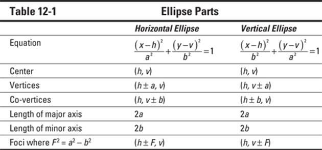
You have to be prepared not only to graph ellipses but also to name all their parts. If a problem asks you to calculate the parts of an ellipse, you have to be ready to deal with some ugly square roots and/or decimals. Table 12-1 presents the parts in a handy, at-a-glance format. This section prepares you to graph and to find all the parts of an ellipse.
Locating vertices and co-vertices
To find the vertices in a horizontal ellipse, use (h ± a, v); to find the co-vertices, use (h, v ± b). A vertical ellipse has vertices at (h, v ± a) and co-vertices at (h ± b, v).
For example, look at this equation, which is already in the proper form to graph:
![]()
You know that h = 5 and v = –1 (switching the signs inside the parentheses). You also know that a2 = 16 (because a has to be the greater number!), or a = 4. If b2 = 9, then b = 3.
This example is a vertical ellipse because the bigger number is under y, so be sure to use the correct formula. This equation has vertices at (5, –1 ± 4), or (5, 3) and (5, –5). It has co-vertices at (5 ± 3, –1), or (8, –1) and (2, –1).
Pinpointing the axes and foci
The major axis in a horizontal ellipse is given by the equation y = v; the minor axis is given by x = h. The major axis in a vertical ellipse is represented by x = h; the minor axis is represented by y = v. The length of the major axis is 2a, and the length of the minor axis is 2b.
You can calculate the distance from the center to the foci in an ellipse (either variety) by using the equation a2 – b2 = F2, where F is the distance from the center to each focus. The foci always appear on the major axis at the given distance (F) from the center.
Using the example from the previous section, you can find the foci with the equation 16 – 9 = F2. The focal distance is ![]() . Because the ellipse is vertical, the foci are at
. Because the ellipse is vertical, the foci are at ![]() .
.
Working with an ellipse in nonstandard form
What if the elliptical equation you’re given isn’t in standard form? Take a look at the example 3x2 + 6x + 4y2 – 16y – 5 = 0. Before you do a single thing, determine that the equation is an ellipse because the coefficients on x2 and y2 are both positive but not equal. Follow these steps to put the equation in standard form:
1. Add the constant to the other side.
This step gives you 3x2 + 6x + 4y2 – 16y = 5.
2. Complete the square.
You need to factor out two different constants now — the different coefficients for x2 and y2:
3(x2 + 2x + 1) + 4(y2 – 4y + 4) = 5
3. Balance the equation by adding the new terms to the other side.
In other words, 3(x2 + 2x + 1) + 4(y2 – 4y + 4) = 5 + 3 + 16.
Note: Adding 1 and 4 inside the parentheses really means adding 3 × 1 and 4 × 4 to each side, because you have to multiply by the coefficient before adding it to the right side.
4. Factor the left side of the equation and simplify the right.
You now have 3(x + 1)2 + 4(y – 2)2 = 24.
5. Divide the equation by the constant on the right to get 1 and then reduce the fractions.
You now have the form ![]() .
.
6. Determine whether the ellipse is horizontal or vertical.
Because the bigger number is under x, this ellipse is horizontal.
7. Find the center and the length of the major and minor axes.
The center is located at (h, v), or (–1, 2).
If a2 = 8, then ![]() .
.
If b2 = 6, then ![]() .
.
8. Graph the ellipse to determine the vertices and co-vertices.
Go to the center first and mark the point. Because this ellipse is horizontal, a moves to the left and right ![]() units (about 2.83) from the center and
units (about 2.83) from the center and ![]() units (about 2.45) up and down from the center. Plotting these points locates the vertices of the ellipse.
units (about 2.45) up and down from the center. Plotting these points locates the vertices of the ellipse.
Its vertices are at ![]() , and its co-vertices are at
, and its co-vertices are at ![]() . The
. The
major axis is at y = 2, and the minor axis is at x = –1. The length of the major axis is ![]() , and the length of the minor axis is
, and the length of the minor axis is ![]() .
.
9. Plot the foci of the ellipse.
You determine the focal distance from the center to the foci in this ellipse with the equation 8 – 6 = F2, so 2 = F2. Therefore, ![]() . The foci, expressed as points, are located at
. The foci, expressed as points, are located at ![]() .
.
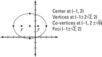
Figure 12-12 shows all the parts of this ellipse in its fat glory.
Figure 12-12:The many points and parts of a horizontal ellipse.
Pair Two Parabolas and What Do You Get? Hyperbolas
Hyperbola literally means “overshooting” in Greek, so it’s a fitting name: A hyperbola is basically “more than a parabola.” Think of a hyperbola as a mix of two parabolas — each one a perfect mirror image of the other each opening away from one another. The vertices of these parabolas are a given distance apart, and they either both open vertically or horizontally.
The mathematical definition of a hyperbola is the set of all points where the difference in the distance from two fixed points (called the foci) is constant. In this section, you discover the ins and outs of the hyperbola, including how to name its parts and graph it.
Visualizing the two types of hyperbolas and their bits and pieces
Similar to ellipses (see the previous section), hyperbolas come in two types: horizontal and vertical.
The equation for a horizontal hyperbola is ![]() .
.
The equation for a vertical hyperbola is ![]() .
.
Notice that x and y switch places (as well as the h and v with them) to name horizontal versus vertical, compared to ellipses, but a and b stay put. So for hyperbolas, a2 always comes first, but it isn’t necessarily greater. More accurately, a is always squared under the positive term (either x2 or y2). Basically, to get a hyperbola into standard form, you need to be sure that the positive squared term is first.
The center of a hyperbola is not actually on the curve itself but exactly in between the two vertices of the hyperbola. Always plot the center first and then count out from the center to find the vertices, axes, and asymptotes.
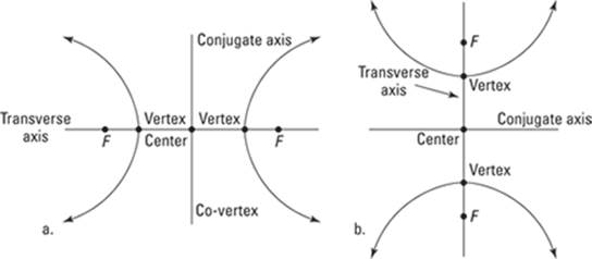
A hyperbola has two axes of symmetry. The one that passes through the center and the two foci is called the transverse axis; the one that’s perpendicular to the transverse axis through the center is called the conjugate axis. A horizontal hyperbola has its transverse axis at y = v and its conjugate axis at x = h; a vertical hyperbola has its transverse axis at x = h and its conjugate axis at y = v.
You can see the two types of hyperbolas in Figure 12-13. Figure 12-13a is a horizontal hyperbola, and Figure 12-13b is a vertical one.
Figure 12-13: A horizontal and a vertical hyperbola, dissected for your viewing pleasure.
If the hyperbola that you’re trying to graph isn’t in standard form, then you need to complete the square to get it into standard form. For the steps of completing the square with conic sections, check out the earlier section “Identifying the min and max on vertical parabolas.”
For example, the following equation is a vertical hyperbola:
![]()
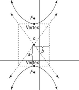
The center (h, v) is (–1, 3). If a2 = 16, a = 4, which means that you count vertical direction (because it is the number under the y variable); and if b2 = 9, then b = 3 (which means that you count horizontally 3 units from the center both to the left and to the right). The distance from the center to the edge of the rectangle marked “a” determines half the length of the transverse axis, and the distance to the edge of the rectangle marked “b” determines the conjugate axis. In a hyperbola, a could be greater than, less than, or equal to b. If you count out a units from the center along the transverse axis and b units from the center in both directions along the conjugate axis, these four points will be the midpoints of the sides of a very important rectangle. This rectangle has sides that are parallel to the x- and y-axis (in other words, don’t just connect the four points, because they’re the midpoints of the sides, not the corners of the rectangle). This rectangle is a useful guide when you need to graph the hyperbola.
But as you can see in Figure 12-13, hyperbolas contain other important parts that you must consider. For instance, a hyperbola has two vertices. Horizontal hyperbolas and vertical hyperbolas have different equations for vertices:
![]() A horizontal hyperbola has vertices at (h ± a, v).
A horizontal hyperbola has vertices at (h ± a, v).
![]() A vertical hyperbola has vertices at (h, v ± a).
A vertical hyperbola has vertices at (h, v ± a).
The vertices for the previous example are at (–1, 3 ± 4), or (–1, 7) and (–1, –1).
You find the foci of any hyperbola by using the equation a2 + b2 = F2, where F is the distance from the center to the foci along the transverse axis, the same axis that the vertices are on. The distance F moves in the same direction as a. Continuing our example, 16 + 9 = F2, or 25 = F2. Taking the root of both sides gives you 5 = F.
To name the foci as points in a horizontal hyperbola, you use (h ± F, v); to name them in a vertical hyperbola, you use (h, v ± F). The foci in the example would be (–1, 3 ± 5), or (–1, 8) and (–1, –2). Note that these points place them inside the hyperbola.
Through the center of the hyperbola and through the corners of the rectangle mentioned previously run the asymptotes of the hyperbola. These asymptotes help guide your sketch of the curves because the curves cannot cross them at any point on the graph. The slopes of these asymptotes are ![]() for a
for a
vertical parabola, or ![]() for a horizontal parabola.
for a horizontal parabola.
Graphing a hyperbola from an equation
To graph a hyperbola, you take all the information from the previous section and put it to work. Follow these simple steps:
1. Mark the center.
Stick with the example hyperbola from the previous section:
![]()
You find that the center of this hyperbola is (–1, 3). Remember to switch the signs of the numbers inside the parentheses, and also remember that h is inside the parentheses with x, and v is inside the parentheses with y. For this example, the quantity with y squared comes first, but h and v don’t switch places. The h and v always remain true to their respective variables, x and y.
2. From the center in Step 1, find the transverse and conjugate axes.
Go up and down the transverse axis a distance of 4 (because 4 is under y), and then go right and left 3 (because 3 is under x). But don’t connect the dots to get an ellipse! Up until now, the steps of drawing a hyperbola were exactly the same as when you drew an ellipse, but here is where things get different: The points you marked as a (on the transverse axis) are your vertices.
3. Use these points to draw a rectangle that will help guide the shape of your hyperbola.
Because you went up and down 4, the height of your rectangle is 8; going left and right 3 gives you a width of 6.
4. Draw diagonal lines through the center and the corners of the rectangle that extend beyond the rectangle.
This step gives you two lines that will be your asymptotes.
5. Sketch the curves.
Beginning at each vertex separately, draw the curves that hug the asymptotes the farther away from the vertices the curve gets.
The graph approaches the asymptotes but never actually touches them.
Figure 12-14 shows the finished hyperbola.
Figure 12-14:Creating a rectangle to graph a hyperbola with asymptotes.
Finding the equation of asymptotes
Because hyperbolas are formed by a curve where the difference of the distances between two points is constant, the curves behave differently than the other conic sections in this chapter. Because distances can’t be negative, the graph has asymptotes that the curve can’t cross over.
Hyperbolas are the only conic sections with asymptotes. Even though parabolas and hyperbolas look very similar, parabolas are formed by the distance from a point and the distance to a line being the same. Therefore, parabolas don’t have asymptotes.
Some pre-calculus problems ask you to find not only the graph of the hyperbola but also the equation of the lines that determine the asymptotes. When asked to find the equation of the asymptotes, your answer depends on whether the hyperbola is horizontal or vertical.
If the hyperbola is horizontal, the asymptotes are given by the line with the
equation ![]() . If the hyperbola is vertical, the asymptotes have
. If the hyperbola is vertical, the asymptotes have
the equation ![]() .
.
The fractions b/a and a/b are the slopes of the lines. You get familiar with point-slope form in Algebra II. Now that you know the slope of your line and a point (which is the center of the hyperbola), you can always write the equations without having to memorize the two asymptote formulas.
Once again, using our example, the hyperbola is vertical so the slope of the asymptotes is ![]() .
.
1. Find the slope of the asymptotes.
Because this hyperbola is vertical, the slopes of the asymptotes are ±4/3.
2. Use the slope from Step 1 and the center of the hyperbola as the point to find the point–slope form of the equation.
Remember that the equation of a line with slope m through point (x1, y1) is y – y1 = m(x – x1). Therefore, if the slope is ±4/3 and the point is (–1, 3),
then the equation of the line is ![]() .
.
3. Solve for y to find the equation in slope-intercept form.
You have to do each asymptote separately here.
• Distribute 4/3 on the right to get ![]() , and then subtract
, and then subtract
3 from both sides to get ![]() .
.
• Distribute –4/3 to the right side to get ![]() . Then subtract
. Then subtract
3 from both sides to get ![]() .
.
Expressing Conics Outside the Realm of Cartesian Coordinates
Up to this point in this chapter, we’ve been graphing conics by using rectangular coordinates (x, y). You may also be asked to graph them in two other ways:
![]() In parametric form: Parametric form is a fancy way of saying a form in which you can deal with conics that aren’t easily expressed as the graph of a function y = f(x). Parametric equations are usually used to describe the motion or velocity of an object with respect to time. Using parametric equations allows you to evaluate both x and y as dependent variables, as opposed to x being independent and y dependent on x.
In parametric form: Parametric form is a fancy way of saying a form in which you can deal with conics that aren’t easily expressed as the graph of a function y = f(x). Parametric equations are usually used to describe the motion or velocity of an object with respect to time. Using parametric equations allows you to evaluate both x and y as dependent variables, as opposed to x being independent and y dependent on x.
![]() In polar form: As you can see in Chapter 11, in polar form every point is (r, θ).
In polar form: As you can see in Chapter 11, in polar form every point is (r, θ).
The following sections show you how to graph conics in these forms.
Graphing conic sections in parametric form
Parametric form defines both the x- and the y-variables of conic sections in terms of a third, arbitrary variable, called the parameter, which is usually represented by t, and you can find both x and y by plugging in t to the parametric equations. As t changes, so do x and y, which means that y is no longer dependent on x but is dependent on t.
Why switch to this form? Consider, for example, an object moving in a plane during a specific time interval. If a problem asks you to describe the path of the object and its location at any certain time, you need three variables:
![]() Time t, which usually is the parameter
Time t, which usually is the parameter
![]() The coordinates (x, y) of the object at time t
The coordinates (x, y) of the object at time t
The xt equation gives the horizontal movement of an object as t changes; the yt equation gives the vertical movement of an object over time.
For example, one set of equations defines both x and y for the same parameter — t — and defines the parameter in a set interval:
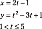 .
.
Time t exists only between 1 and 5 seconds for this problem.
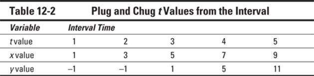
If you’re asked to graph this equation, you can do it in one of two ways. The first method is the plug and chug: Set up a chart and pick t values from the given interval in order to figure out what x and y should be, and then graph these points like normal. Table 12-2 shows the results of this process. Note: We include t = 1 in the chart, even though the parameter isn’t defined there. You need to see what it would’ve been, because you graph the point where t = 1 with an open circle to show what happens to the function arbitrarily close to 1. Be sure to make that point an open circle on your graph.
The other way to graph a parametric curve is to solve one equation for the parameter and then substitute that equation into the other equation. You should pick the simplest equation to solve and start there.
Sticking with the same example, solve the linear equation x = 2t – 1 for t:
1. Solve the simplest equation.
For the chosen equation, you get ![]() .
.
2. Plug the solved equation into the other equation.
For this step, you get ![]() .
.
3. Simplify this equation if necessary.
You now have ![]() .
.
Because this step gives you an equation in terms of x and y, you can graph the points on the coordinate plane just like you always do. The only problem is that you don’t draw the entire graph, because you have to look at a specific interval of t.
4. Substitute the endpoints of the t interval into the x function to know where the graph starts and stops.
We do this in Table 12-2. When t = 1, x = 1, and when t = 5, x = 9.
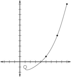
Figure 12-15 shows the parametric curve from this example (for both methods). You end up with a parabola, but you can also write parametric equations for ellipses, circles, and hyperbolas.
Figure 12-15:Graphing a parametric curve.
If you have a graphing calculator, you can set it to parametric mode to graph. When you go into your graphing utility, you get two equations — one is “x =” and the other is “y =.” Input both equations exactly as they’re given, and the calculator will do the work for you!
The equations of conic sections on the polar coordinate plane
Graphing conic sections on the polar plane (see Chapter 11) is based on equations that depend on a special value known as eccentricity, which describes the overall shape of a conic section. The value of a conic’s eccentricity can tell you what type of conic section the equation describes, as well as how fat or skinny it is. When graphing equations in polar coordinates, you may have trouble telling which conic section you should be graphing based solely on the equation (unlike graphing in Cartesian coordinates, where each conic section has its own unique equation). Therefore, you can use the eccentricity of a conic section to find out exactly which type of curve you should be graphing.
Here are the two equations that allow you to put conic sections in polar coordinate form, where (r, θ) is the coordinate of a point on the curve in polar form. Recall from Chapter 11 that r is the radius, and θ is the angle in standard position on the polar coordinate plane.
![]() or
or ![]()
![]() or
or ![]()
When graphing conic sections in polar form, you can plug in various values of θ to get the graph of the curve. In each equation above, k is a constant value, θ takes the place of time, and e is the eccentricity. The variable edetermines the conic section:
![]() If e = 0, the conic section is a circle.
If e = 0, the conic section is a circle.
![]() If 0 < e < 1, the conic section is an ellipse.
If 0 < e < 1, the conic section is an ellipse.
![]() If e = 1, the conic section is a parabola.
If e = 1, the conic section is a parabola.
![]() If e > 1, the conic section is a hyperbola.
If e > 1, the conic section is a hyperbola.
For example, say you want to graph this equation:
![]()
First realize that as it’s shown, it doesn’t fit the form of any of the equations we have introduced you to for the conic sections. It doesn’t fit because all the denominators of the conic sections begin with 1, and this equation begins with 4. Have no fear; you can factor out that 4, which then tells you what k is!
Factoring out the 4 from the denominator gives you 1 – e cosθ. In order to keep the equation as close to the standard form for polar conics, multiply the
numerator and denominator by 1/4. This step gives you 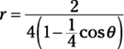 ,
,
which is the same as 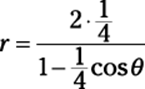 .
.
Therefore, the constant k is 2 and the eccentricity, e, is 1/4, which tells you that you have an ellipse because e is between 0 and 1.
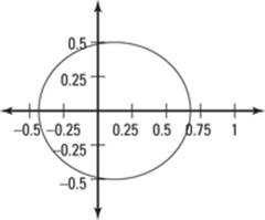
In order to graph the polar function of the ellipse mentioned above, you can plug in values of θ and solve for r. Then plot the coordinates of (r, θ) on the polar coordinate plane to get the graph. For the graph of the previous equation,
![]() , you can plug in 0,
, you can plug in 0, ![]() , π, and
, π, and ![]() , and find r:
, and find r:
r(0): The cosine of 0 is 1, so ![]() .
.
![]() : The cosine of
: The cosine of ![]() is 0, so
is 0, so ![]() .
.
r(π): The cosine of π is –1, so ![]() .
.
![]() : The cosine of
: The cosine of ![]() is 0, so
is 0, so ![]() .
.
These four points are enough to give you a rough sketch of the graph. You can see the graph of the example ellipse in Figure 12-16.
Figure 12-16:The graph of an ellipse in polar coordinates.