Pre-Calculus For Dummies, 2nd Edition (2012)

Part I. Set It Up, Solve It, Graph It

Chapter 3. The Building Blocks of Pre-Calc: Functions

In This Chapter

Identifying, graphing, and translating parent functions

Piecing together piece-wise functions

Breaking down and graphing rational functions

Performing different operations on functions

Maps of the world identify cities as dots and use lines to represent the roads that connect them. Modern country and city maps use a grid system to help users find locations easily. If you can’t find the place you’re looking for, you look at an index, which gives you a letter and number. This information narrows down your search area, after which you can easily figure out how to get where you’re going.

You can take this idea and use it for your own pre-calc purposes through the process of graphing. But instead of naming cities, the dots name points on the coordinate plane (which we discuss more in Chapter 1). A point on this plane relates two numbers to each other, usually in the form of input and output. The whole coordinate plane really is just a big computer, because it’s based on input and output, with you as the operating system. This idea of input and output is best expressed mathematically using functions. A function is a set of ordered pairs where every x value gives one and only one y value (as opposed to a relation).

This chapter shows you how to perform your role as the operating system, explaining the map of the world of points and lines on the coordinate plane along the way.

Qualities of Even and Odd Functions and Their Graphs

Knowing whether a function is even or odd helps you to graph it because that information tells you which half of the points you have to graph. These types of functions are symmetrical, so whatever is on one side is exactly the same as the other side. If a function is even, the graph is symmetrical over the y-axis. If the function is odd, the graph is symmetrical about the origin.

Even function: The mathematical definition of an even function is f(–x) = f(x) for any value of x. The simplest example of this is f(x) = x²; f(3) = 9, and f(–3) = 9. Basically, the opposite input yields the same output. Visually speaking, the graph is a mirror image across the y-axis.

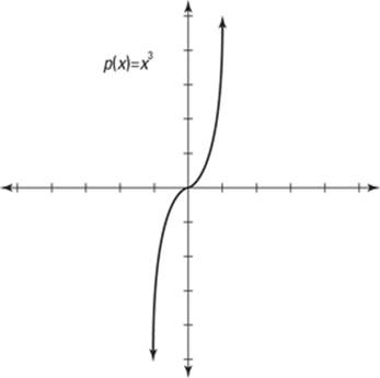
Odd function: The definition of an odd function is f(–x) = –f(x) for any value of x. The opposite input gives the opposite output. These graphs have 180-degree symmetry about the origin. If you turn the graph upside down, it looks the same. For example, f(x) = x³ is an odd function because f(3) = 27 and f(–3) = –27.

Dealing with Parent Functions and Their Graphs

In mathematics, you see certain graphs over and over again. For that reason, these original, common functions are called the parent graphs, and they include graphs of quadratic functions, square roots, absolute value, cubics, and cube roots. In this section, we work to get you used to graphing the parent graphs so you can graduate to more in-depth graphing work.

Quadratic functions

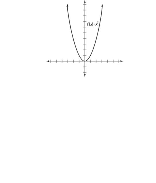
Quadratic functions are equations in which the 2nd power, or square, is the highest to which the unknown quantity or variable is raised. In such an equation, either x or y is squared, but not both. The graph of x = y²isn’t a function, because any positive x value produces two different y values — look at (4, 2) and (4, –2) for example. The equation y or f(x) = x² is a quadratic function and is the parent graph for all other quadratic functions.

The shortcut to graphing the function f(x) = x² is to start at the point (0, 0) (the origin) and mark the point, called the vertex. Note that the point (0, 0) is the vertex of the parent function only — later, when you transform graphs, the vertex moves around the coordinate plane. In calculus, this point is called a critical point, and some pre-calc teachers also use that terminology. Without getting into the calc definition, it means that the point is special.

The graph of any quadratic function is called a parabola. All parabolas have the same basic shape (for more, see Chapter 12). To get the other points, you move 1 horizontally from the vertex, up 1², over 2, up 2², over 3, up 3², and so on. This graphing occurs on both sides of the vertex and keeps going, but usually just a couple points on either side of the vertex gives you a good idea of what the graph looks like. Check out Figure 3-1 for an example of a quadratic function in graph form.

Square-root functions

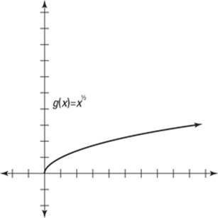
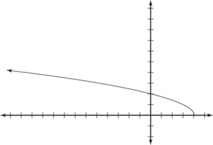
A square-root graph is related to a quadratic graph (see the previous section). The quadratic graph is f(x) = x², whereas the square-root graph is g(x) = x^1/2. The graph of a square-root function looks like the left half of a parabola that has been rotated 90 degrees clockwise. You can also write the square-root function as .

However, only half of the parabola exists, for two reasons. Its parent graph exists only when x is zero or positive (because you can’t find the square root of negative numbers [and keep them real, anyway]) and when g(x) is positive (because when you see , you’re being asked to find only the principal or positive root when x > 0).

This graph starts at the origin (0, 0) and then moves to the right 1 position, up (1); to the right 2, up ; to the right 3, up ; and so on. Check out Figure 3-2 for an example of this graph.

Notice that the values you get by plotting consecutive points don’t exactly give you the nicest numbers. Instead, try picking values for which you can easily find the square root. Here’s how this works: Start at the origin and go right 1, up (1); right 4, up (2); right 9, up (3); and so on.

Absolute-value functions

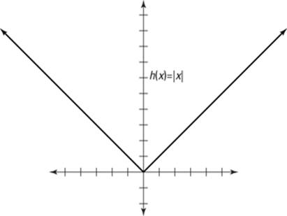
The absolute-value parent graph of the function y = |x| turns all inputs non-­negative (0 or positive). To graph absolute-value functions, you start at the origin and move in both directions along the x-axis and the y-axis from there: over 1, up 1; over 2, up 2; and on and on forever. Figure 3-3 shows this graph in action.

Cubic functions

In a cubic function, the highest degree on any variable is three — f(x) = x³ is the parent function. You start graphing the cubic function parent graph at its critical point, which is also the origin (0, 0). The origin isn’t, however, a critical point for every function.

From the critical point, the cubic graph moves right 1, up 1³; right 2, up 2³; and so on. The function x³ is an odd function, so you rotate half of the graph 180 degrees about the origin to get the other half. Or, you can move left –1, down (–1)³; left –2, down (–2)³; and so on. How you plot is based on your personal preference. Consider g(x) = x³ in Figure 3-4.

Cube-root functions

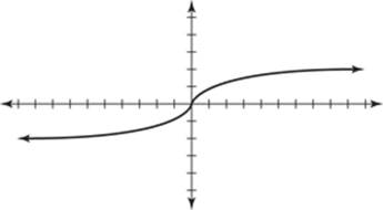
Cube-root functions are related to cubic functions in the same way that square-root functions are related to quadratic functions. You write cubic functions as f(x) = x³ and cube-root functions as g(x) = x^1/3 or .

Noting that a cube-root function is odd is important because it helps you graph it. The critical point of the cube-root parent graph is at the origin (0, 0), as shown in Figure 3-5.

Transforming the Parent Graphs

In certain situations, you need to use a parent function to get the graph of a more complicated version of the same function. For instance, you can graph each of the following by transforming its parent graph:

f(x) = –2(x + 1)² – 3

h(x) = (x – 1)⁴ + 2

As long as you have the graph of the parent function, you can transform it by using the rules we describe in this section. When using a parent function for this purpose, you can choose from the following different types of transformations (discussed in more detail in the following sections):

Vertical transformations cause the parent graph to stretch or shrink ­vertically.

Horizontal transformations cause the parent graph to stretch or shrink horizontally.

Translations cause the parent graph to shift left, right, up, or down (or a combined shift both horizontally and vertically).

Reflections flip the parent graph over a horizontal or vertical line. They do just what their name suggests: mirror the parent graphs (unless other transformations are involved, of course).

The methods to transform quadratic functions also work for all other types of common functions, such as square roots. A function is always a function, so the rules for transforming functions always apply, no matter what type of function you’re dealing with.

And if you can’t remember these shortcut methods later on, you can always take the long route: picking random values for x and plugging them into the function to see what y values you get.

Vertical transformations

A number (or coefficient) multiplying in front of a function causes a vertical transformation, a fancy math term for change in height. The coefficient always affects the height of each and every point in the graph of the function. We call the vertical transformation a stretch if the coefficient is greater than 1 and a shrink if the coefficient is between 0 and 1.

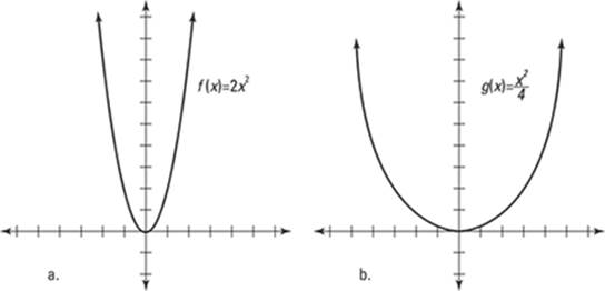
For example, the graph of f(x) = 2x² takes the graph of f(x) = x² and stretches it by a vertical factor of two. That means that each time you plot a point vertically on the graph, the value gets multiplied by two (making the graph twice as tall at each point). So from the vertex, you move over 1, up 2 · 1² (= 2); over 2, up 2 · 2² (= 8); over 3, up 2 · 3² (= 18); and so on. Figure 3-6 shows two different graphs to illustrate vertical transformation.

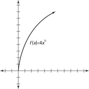
The transformation rules apply to any function, so Figure 3-7, for instance, shows . The 4 is a vertical stretch; it makes the graph four times as tall at every point: right 1, up (= 4); right 4, up (notice that we’re using numbers that you can easily take the square root of to make graphing a simple task); and so on.

Horizontal transformations

Horizontal transformation means to stretch or shrink a graph along the x-axis. A number multiplying a variable inside a function affects the horizontal position of the graph — a little like the fast-forward or slow-motion button on a remote control, making the graph move faster or slower. A coefficient greater than 1 causes the function to stretch horizontally, making it appear to move faster. A coefficient between 0 and 1 makes the function appear to move slower, or a horizontal shrink.

For instance, look at the graph of f(x) = |2x| (see Figure 3-8). The distance between any two consecutive values from the parent graph |x| along the x-axis is always 1. If you set the inside of the new, transformed function equal to the distance between the x values, you get 2x = 1. Solving the equation gives you x = 1/2, which is how far you step along the x-axis. Beginning at the origin (0, 0), you move right 1/2, up 1; right 1, up 2; right 3/2, up 3; and so on.

Translations

Moving a graph horizontally or vertically is called a translation. In other words, every point on the parent graph is translated left, right, up, or down. In this section, you find information on both kinds of translations: horizontal shifts and vertical shifts.

Horizontal shifts

A number adding or subtracting inside the parentheses (or other grouping device) of a function creates a horizontal shift. Such functions are written in the form f(x – h), where h represents the horizontal shift.

The numbers in this function do the opposite of what they look like they should do. For example, if you have the equation g(x) = (x – 3)², the graph moves to the right three units; in h(x) = (x + 2)², the graph moves to the left two units.

Why does it work this way? Examine the parent function f(x) = x² and the horizontal shift g(x) = (x – 3)². When x = 3, f(3) = 3² = 9 and g(3) = (3 – 3)² = 0² = 0. The g(x) function acts like the f(x) function when x was 0. In other words, f(0) = g(3). It’s also true that f(1) = g(4). Each point on the parent function gets moved to the right by three units; hence, three is the horizontal shift for g(x).

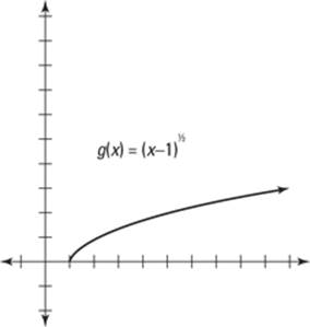
Try your hand at graphing . Because – 1 is underneath the square root sign, this shift is horizontal — the graph gets moved to the right one position. If (the parent function), you’ll find that k(0) = g(1), which is to the right by one. Figure 3-9 shows the graph of g(x).

Vertical shifts

Adding or subtracting numbers completely separate from the function causes a vertical shift in the graph of the function. Consider the expression f(x) + v, where v represents the vertical shift. Notice that the addition of the variable exists outside the function.

Vertical shifts are less complicated than horizontal shifts (see the previous section), because reading them tells you exactly what to do. In the equation f(x) = x² – 4, you can probably guess what the graph is going to do: It moves down four units, whereas the graph of g(x) = x² + 3 moves up three.

Note: You see no vertical stretch or shrink for either f(x) or g(x), because the coefficient in front of x² for both functions is 1. If another number multiplied with the functions, you’d have a vertical stretch or shrink.

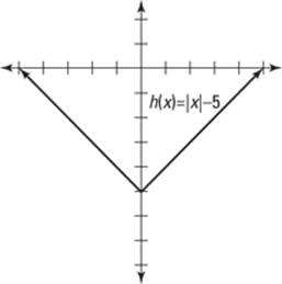
To graph the function h(x) = |x| – 5, notice that the vertical shift is down five units. Figure 3-10 shows this translated graph.

When translating a cubic function, the critical point moves horizontally or vertically, so the point of symmetry around which the graph is based moves as well. In the function f(x) = x³ – 4 in Figure 3-11, for instance, the point of symmetry is (0, –4).

Reflections

Reflections take the parent function and provide a mirror image of it over either a horizontal or vertical line. You’ll come across two types of reflections:

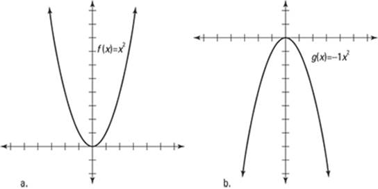
A negative number multiplies the whole function (as in ): The negative outside the function reflects over a horizontal line because it makes the output value negative if it was positive and positive if it was negative. Look at Figure 3-12, which shows the parent function f(x) = x² and the reflection g(x) = –1x². If you find the value of both functions at the same number in the domain, you’ll get opposite values in the range. For example, if x = 4, f(4) = 16 and g(4) = –16.

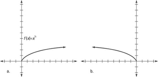
A negative number multiplies only the input x (as in ): Vertical reflections work the same as horizontal reflections, except the reflection occurs across a vertical line and reflects from side to side rather than up and down. You now have a negative inside the function. For this reflection, evaluating opposite inputs in both functions yields the same output. For example, if , you can write its reflection over a vertical line as . When f(4) = 2, g(–4) = 2 as well (check out the graph in Figure 3-13).

Combining various transformations (a transformation in itself!)

Certain mathematical expressions allow you to combine stretching, shrinking, translating, and reflecting a function all into one graph. An expression that shows all the transformations in one is , where

a is the vertical transformation.

c is the horizontal transformation.

h is the horizontal shift.

v is the vertical shift.

For instance, f(x) = –2(x – 1)² + 4 moves right 1 and up 4, stretches twice as tall, and reflects upside down. Figure 3-14 shows each stage.

Figure 3-14a is the parent graph: k(x) = x².

Figure 3-14b is the horizontal shift to the right by one: h(x) = (x – 1)².

Figure 3-14c is the vertical shift up by four: g(x) = (x – 1)² + 4.

Figure 3-14d is the vertical stretch of two: f(x) = –2(x – 1)² + 4. (Notice that because the value was negative, the graph was also turned upside down.)

Allow us to show one more transformation — and illustrate the importance

of the order of the process. You graph the function with the following steps:

1. Rewrite the function in the form .

Reorder the function so that the x comes first (in descending

order). And don’t forget the negative sign! Here it is: .

2. Factor out the coefficient in front of the x.

You now have .

3. Reflect the parent graph.

Because the –1 is inside the square-root function, q(x) is a horizontal reflection over a vertical line of .

4. Shift the graph.

The factored form of q(x) (from Step 2) reveals that the horizontal shift is four to the right.

Figure 3-15 shows the graph of q(x).

Transforming functions point by point

For some problems, you may be required to transform a function given only a set of random points on the coordinate plane. Quite frankly, your textbook or teacher will be making up some new kind of function that has never existed before. Just remember that all functions follow the same transformation rules, not just the common functions that we’ve explained so far in this chapter.

For example, the graphs of y = f(x) and are shown in Figure 3-16.

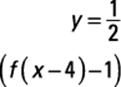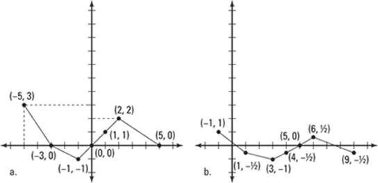
Figure 3-16a represents the parent function (the set of random points). Figure 3-16b transforms the parent function by shrinking it by a factor of 1/2 and then translating it to the right four units and down one unit. The first random point on the parent function is (–5, 3); shifting it to the right by four puts you at (–1, 3), and shifting it down one puts you at (–1, 2). Because the translated height is two, you shrink the function by finding 1/2 of 2. You end up at the final point, which is (–1, 1).

You must repeat that process for as many points as you see on the original graph to get the transformed one.

Graphing Functions that Have More than One Rule: Piece-Wise Functions

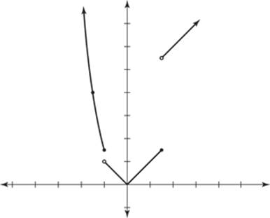
Piece-wise functions are functions broken into pieces, depending on the input. A piece-wise function has more than one function, but each function is defined only on a specific interval. Basically, the output depends on the input, and the graph of the function sometimes looks like it’s literally been broken into pieces.

For example, the following represents a piece-wise function:

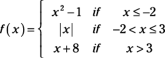
This function is broken into three pieces, depending on the domain values for each piece:

The first piece is the quadratic function f(x) = x² – 1 and exists only on the interval (–∞, –2]. As long as the input for this function is less than –2, the function exists in the first piece (the top line) only.

The second piece is the absolute-value function f(x) = |x| and exists only on the interval (–2, 3].

The third piece is the linear function f(x) = x + 8 and exists only on the interval (3, ∞).

To graph this example function, follow these steps:

1. Lightly sketch out a quadratic function that moves down one (see the earlier section “Quadratic functions”) and darken all the values to the left of x = –2.

Because of the interval of the quadratic function of the first piece, you darken all points to the left of –2. And because x = –2 is included (the interval is x ≤ –2), the circle at x = –2 is filled in.

2. Between –2 and 3, the graph moves to the second function of the equation (|x| if 2 < x ≤ 3); sketch the absolute-value graph (see the earlier section “Absolute-value functions”), but pay attention only to the xvalues between –2 and 3.

You don’t include –2 (open circle), but the 3 is included (closed circle).

3. For x values bigger than 3, the graph follows the third function of the equation: x + 8 if x > 3.

You sketch in this linear function where b = 4 with a slope of 1, but only to the right of x = 3 (that point is an open circle). The finished product is shown in Figure 3-17.

Notice that you can’t draw the graph of this piece-wise function without lifting your pencil from the paper. Mathematically speaking, this is called a discontinuous function. You get to practice discontinuities with rational functions later in this chapter.

Calculating Outputs for Rational Functions

In addition to the common parent functions, you have to graph another type of function in pre-calculus: rational functions, which basically are functions where the variable appears in the denominator of a fraction. (This situation isn’t the same as the rational exponents you see in Chapter 2, though. The word rational means fraction; in Chapter 2 we deal with fractions as exponents, and now they’re the entire function.)

The mathematical definition of a rational function is a function that can be expressed as the quotient of two polynomials, such that

where the degree of q(x) is greater than zero.

The variable in the denominator of a rational function could create a situation where the denominator is zero for certain numbers in the domain. Of course, division by zero is an undefined value in mathematics. Typically in a rational function, you find at least one value of x for which the rational function is undefined, at which point the graph will have an asymptote — the graph gets closer and closer to that value but never crosses it (in the case of vertical asymptotes). Knowing in advance that these values of x are undefined helps you to graph.

In the following sections, we show you the steps involved in finding the outputs of (and ultimately graphing) rational functions.

Step 1: Search for vertical asymptotes

Having the variable on the bottom of a fraction is a problem, because the denominator of a fraction can never be zero. Usually, some domain value(s) of x makes the denominator zero. The function “jumps over” this value in the graph, creating what’s called a vertical asymptote. Graphing the vertical asymptote first shows you the number in the domain where your graph can’t pass through. The graph approaches this point but never reaches it. With that in mind, what value(s) for x can you not plug into the rational function?

The following equations are all rational:

Try to find the value for x in which the function is undefined. Use the following steps to find the vertical asymptote for f(x) first:

1. Set the denominator of the rational function equal to zero.

For f(x), x² + 4x – 21 = 0.

2. Solve this equation for x.

Because this equation is a quadratic (see the earlier section “Quadratic functions” and Chapter 4), try to factor it. This quadratic factors to (x + 7)(x – 3) = 0. Set each factor equal to zero to solve. If x + 7 = 0, x = –7. If x – 3 = 0, x = 3. Your two vertical asymptotes, therefore, are x = –7 and x = 3.

Now you can find the vertical asymptote for g(x). Follow the same set of steps:

4 – 3x = 0

x = 4/3

Now you have your vertical asymptote for g(x). That was easy! Time to do it all again for h(x):

x + 2 = 0

x = –2

Keep these equations for the vertical asymptotes close by because you need them when you graph later.

Step 2: Look for horizontal asymptotes

To find a horizontal asymptote of a rational function, you need to look at the degree of the polynomials in the numerator and the denominator. The degree is the highest power of the variable in the polynomial expression. Here’s how you proceed:

If the denominator has the bigger degree (like in the f(x) example in the previous section), the horizontal asymptote automatically is the x-axis, or y = 0.

If the numerator and denominator have an equal degree, you must divide the leading coefficients (the coefficients of the terms with the highest degrees) to find the horizontal asymptote.

Be careful! Sometimes the terms with the highest degrees aren’t written first in the polynomial. You can always rewrite both polynomials so that the highest degrees come first, if you prefer. For instance, you can rewrite the denominator of g(x) as –3x + 4 so that it appears in descending order.

The function g(x) has equal degrees on top and bottom. To find the horizontal asymptote, divide the leading coefficients on the highest-degree terms: y = 6 ÷ –3, or y = –2. You now have your horizontal asymptote for g(x). Hold on to that equation for graphing!

If the numerator has the bigger degree of exactly one more than the denominator, the graph will have an oblique asymptote; see Step 3 for more information on how to proceed.

Step 3: Seek out oblique asymptotes

Oblique asymptotes are neither horizontal nor vertical. In fact, an asymptote doesn’t even have to be a straight line at all; it can be a slight curve or a really complicated curve.

To find an oblique asymptote, you have to use long division of polynomials to find the quotient. You take the denominator of the rational function and divide it into the numerator. The quotient (neglecting the remainder) gives you the equation of the line of your oblique asymptote.

We cover long division of polynomials in Chapter 4. You must understand long division of polynomials in order to complete the graph of a rational function with an oblique asymptote.

The h(x) example from Step 1 has an oblique asymptote because the numerator has the higher degree in the polynomial. By using long division, you get a quotient of x – 2. This quotient means the oblique asymptote follows the equation y = x – 2. Because this equation is first-degree, you graph it by using the slope-intercept form. Keep this oblique asymptote in mind, because graphing is coming right up!

Step 4: Locate the x- and y-intercepts

The final piece of the puzzle is to find the intercepts (where the line or curve crosses the x- and y-axes) of the rational function, if any exist:

To find the y-intercept of an equation, set x = 0. (Plug in 0 wherever you see x.) The y-intercept of f(x) from Step 1, for instance, is 1/21.

To find the x-intercept of an equation, set y = 0.

For any rational function, the shortcut is to set the numerator equal to zero and then solve. Sometimes when you do this, however, the equation you get is unsolvable, which means that the rational function doesn’t have an x-intercept.

The x-intercept of f(x) is 1/3.

Now find the intercepts for g(x) and h(x) from Step 1. Doing so, you find the following points:

g(x) has a y-intercept at 3 and an x-intercept at –2.

h(x) has a y-intercept at –9/2 and x-intercepts at ±3.

Putting the Output to Work: Graphing Rational Functions

After you calculate all the asymptotes and the x- and y-intercepts for a rational function (we take you through that process in the preceding section), you have all the information you need to start graphing the rational function. Graphing a rational function is all about the degree of the numerator and denominator. Because the numerator and the denominator are polynomials, their degrees are easy to find — just look for the highest exponent in each.

Rational functions come in three types, depending on the degree:

The denominator has the greater degree.

The numerator and the denominator have equal degrees.

The numerator has the greater degree.

The following sections describe how to graph in each case.

The denominator has the greater degree

Rational functions are really just fractions. If you look at several fractions where the numerator stays the same but the denominator gets bigger, the whole fraction gets smaller. For instance, look at 1/2, 1/20, 1/200, and 1/2,000.

In any rational function where the denominator has a greater degree as values of x get infinitely large, the fraction gets infinitely smaller until it approaches zero (this process is called a limit; you can see it again in Chapter 15). The following sections break down graphing this type of function.

Graphing the info you know

When the denominator has the greater degree, you begin by graphing the information that you know for f(x). Here we stick with the function from “Step 1: Search for vertical asymptotes”:

Figure 3-18 shows all the parts of the graph:

1. Draw the vertical asymptote(s).

Whenever you graph asymptotes, be sure to use dotted lines, not solid lines, because the asymptotes aren’t part of the rational function.

For f(x), you find that the vertical asymptotes are x = –7 and x = 3, so draw two dotted vertical lines, one at x = –7 and another at x = 3.

2. Draw the horizontal asymptote(s).

Continuing with the example, the horizontal asymptote is y = 0 — or the x-axis.

3. Plot the x-intercept(s) and the y-intercept(s).

The y-intercept is y = 1/21, and the x-intercept is x = 1/3.

Filling in the blanks by plotting outputs of test values

The vertical asymptotes divide the graph and the domain of f(x) into three intervals: (–∞, –7), (–7, 3), and (3, ∞). For each of these three intervals, you must pick at least one test value and plug it into the original rational function; this test determines whether the graph on that interval is above or below the horizontal asymptote (the x-axis). Follow these steps:

1. Test a value in the first interval.

In the example, the first interval is (–∞, –7), so you can choose any number you want as long as it’s less than –7. We choose x = –8 for this example, so now you evaluate

This negative value tells you that the function is under the horizontal asymptote on the first interval only.

2. Test a value in the second interval.

If you look at the second interval (–7, 3) in Figure 3-18, you’ll realize that you already have two test points located in it. The y-intercept has a positive value, which tells you that the graph is above the horizontal asymptote for that part of the graph.

Now here comes the curve ball: It stands to reason that a graph should never cross an asymptote; it should just get closer and closer to it. In this case, there’s an x-intercept, which means that the graph actually crosses its own horizontal asymptote. The graph becomes negative for the rest of this interval.

Sometimes the graphs of rational functions cross a horizontal asymptote, and sometimes they don’t. In this case, where the denominator has a greater degree, and the horizontal asymptote is the x-axis, it depends on whether the function has roots or not. You can find out by setting the numerator equal to zero and solving the equation. If you find a solution, there is a zero and the graph will cross the x-axis. If not, the graph doesn’t cross the x-axis.

Vertical asymptotes are the only asymptotes that are never crossed. A horizontal asymptote actually tells you what value the graph is approaching for infinitely large or negative values of x.

3. Test a value in the third interval.

For the third interval, (3 ∞), we use the test value of 4 (you can use any number greater than 3) to determine the location of the graph on the interval. We get f(4) = 1, which tells you that the graph is above the horizontal asymptote for this last interval.

Knowing a test value in each interval, you can plot the graph by starting at a test value point and moving from there toward both the horizontal and vertical asymptotes. Figure 3-19 shows the complete graph of f(x).

The numerator and denominator have equal degrees

Rational functions with equal degrees in the numerator and denominator behave the way that they do because of limits (see Chapter 15). What you need to remember is that the horizontal asymptote is the quotient of the leading coefficients of the top and the bottom of the function (see the earlier section “Step 2: Look for horizontal asymptotes” for more info).

Take a look at — which has equal degrees on the variables for

each part of the fraction. Follow these simple steps to graph g(x), which is shown in Figure 3-20:

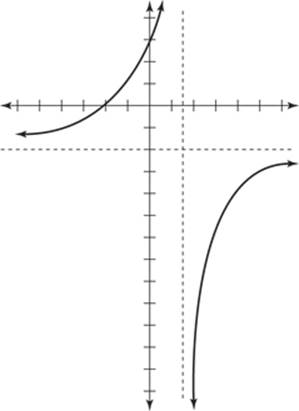
1. Sketch the vertical asymptote(s) for g(x).

From your work in the previous section, you find only one vertical asymptote at x = 4/3, which means you have only two intervals to consider: (–∞, 4/3) and (4/3, ∞).

2. Sketch the horizontal asymptote for g(x).

You find in Step 2 from the previous section that the horizontal asymptote is y = –2. So you sketch a horizontal line at that position.

3. Plot the x- and y-intercepts for g(x).

You find in Step 4 from the previous section that the intercepts are x = –2 and y = 3.

4. Use test values of your choice to determine whether the graph is above or below the horizontal asymptote.

The two intercepts are already located on the first interval and above the horizontal asymptote, so you know that the graph on that entire interval is above the horizontal asymptote (you can easily see that g(x) can never equal to –2). Now, choose a test value for the second interval greater than 4/3. We choose x = 2. Substituting this into the function g(x) gives you –12. You know that –12 is way under –2, so you know that the graph lives under the horizontal asymptote in this second interval.

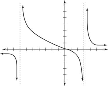
The numerator has the greater degree

Rational functions where the numerator has the greater degree don’t actually have horizontal asymptotes. If the degree of the numerator of a rational function is exactly one more than the degree of its denominator, it has an oblique asymptote, which you find by using long division (see Chapter 4).

It’s time to graph h(x), which is :

1. Sketch the vertical asymptote(s) of h(x).

You find only one vertical asymptote for this rational function — x = –2. And because the function has only one vertical asymptote, you find only two intervals for this graph — (–∞, –2) and (–2, ∞).

2. Sketch the oblique asymptote of h(x).

Because the numerator of this rational function has the greater degree, the function has an oblique asymptote. Using long division, you find that the oblique asymptote follows the equation y = x – 2.

3. Plot the x- and y-intercepts for h(x).

You find that the x-intercepts are ±3 and the y-intercept is –9/2.

4. Use test values of your choice to determine whether the graph is above or below the oblique asymptote.

Notice that the intercepts conveniently give test points in each interval. You don’t need to create your own test points, but you can if you really want to. In the first interval, the test point (–3, 0), hence the graph, is located above the oblique asymptote. In the second interval, the test points (0, –9/2) and (3, 0), as well as the graph, are located under the oblique asymptote.

Figure 3-21 shows the complete graph of h(x).

Sharpen Your Scalpel: Operating on Functions

Yes, graphing functions is fun, but what if you want more? Well, good news; you also can operate with functions. That’s right, we’re here to show you how to add, subtract, multiply, or divide two or more functions.

Operating on (sometimes called combining) functions is pretty easy, but the graphs of new, combined functions can be hard to create, because those combined functions don’t have parent functions and, therefore, no transformations of parent functions that allow you to graph easily. So we steer clear of them in pre-calculus . . . well, except for maybe a few. If you’re asked to graph a combined function, you must resort to the old plug-and-chug method (or perhaps your teacher will be nice enough to let you use your graphing calculator).

This section walks you through various operations you may be asked to perform on functions, using the following three functions throughout the examples:

Adding and subtracting

When asked to add functions, you simply combine like terms, if the functions have any. For example, (f + g)(x) is asking you to add the f(x) and the g(x) functions:

(f + g)(x) = (x² – 6x + 1) + (3x² – 10)

= 4x² – 6x – 9

The x² and 3x² add to 4x²; –6x remains because it has no like terms; 1 and –10 add to –9.

But what do you do if you’re asked to add (g + h)(x)? You get the following equation:

You have no like terms to add, so you can’t simplify the answer any further. You’re done!

When asked to subtract functions, you distribute the negative sign throughout the second function, using the distributive property (see Chapter 1), and then treat the process like an addition problem:

(g – f)(x) = (3x² – 10) – (x² – 6x + 1)

= (3x² – 10) + (–x² + 6x – 1)

= 2x² + 6x – 11

Multiplying and dividing

Multiplying and dividing functions is a similar concept to adding and subtracting them (see the previous section). When multiplying functions, you use the distributive property over and over and then add the like terms to simplify. Dividing functions is trickier, however. We tackle multiplication first and save the trickster division for last. Here’s the setup for multiplying f(x) and g(x):

(fg)(x) = (x² – 6x + 1)(3x² – 10)

Follow these steps to multiply these functions:

1. Distribute each term of the polynomial on the left to each term of the polynomial on the right.

You start with x²(3x²) + x²(–10) + –6x(3x²) + –6x(–10) + 1(3x²) + 1(–10).

You end up with 3x⁴ – 10x² – 18x³ + 60x + 3x² – 10.

2. Combine like terms to get the final answer to the multiplication.

This simple step gives you 3x⁴ – 18x³ – 7x² + 60x – 10.

Operations that call for division of functions may involve factoring to cancel out terms and simplify the fraction. (If you’re unfamiliar with this concept, check out Chapter 4.) If you’re asked to divide g(x) by f(x), though, you write the following equation:

Because neither the denominator nor the numerator factor, the new, combined function is simplified and you’re done.

You may be asked to find a specific value of a combined function. For example, (f + h)(1) asks you to put the value of 1 into the combined function

. When you plug in 1, you get

Breaking down a composition of functions

A composition of functions is one function acting upon another. Think of it like putting one function inside of the other — f(g(x)), for instance, means that you plug the entire g(x) function into f(x). To solve such a problem, you work from the inside out:

f(g(x)) = f(3x² – 10) = (3x² – 10)² – 6(3x² – 10) + 1

This process puts the g(x) function into the f(x) function everywhere the f(x) function asks for x. This equation ultimately simplifies to 9x⁴ – 78x² + 161, in case you’re asked to simplify the composition.

Likewise, , which easily simplifies to 3(2x – 1) – 10 because the square root and square cancel each other. This equation simplifies even further to 6x – 13.

You may also be asked to find one value of a composed function. To find , for instance, it helps to realize that it’s like reading Hebrew: You work from right to left. In this example, you’re asked to put –3 into f(x), get an answer, and then plug that answer into g(x). Here are these two steps in action:

f(–3) = (–3)² – 6(–3) + 1 = 28

g(28) = 3(28)² – 10 = 2,342

Adjusting the domain and range of ­combined functions (if applicable)

If you’ve looked over the previous sections that cover adding, subtracting, multiplying, and dividing functions, or putting one function inside of another, you may be wondering whether all these operations are messing with domain and range. Well, the answer depends on the operation performed and the original function. But yes, the possibility does exist that the domain and range will change when you combine functions.

Following are the two main types of functions whose domains are not all real numbers:

Rational functions: The denominator of a fraction can never be zero, so at times rational functions are undefined.

Square-root functions (and any root with an even index): The radicand (the stuff underneath the root symbol) can’t be negative. To find out how the domain is affected, set the radicand greater than or equal to zero and solve. This solution will tell you the effect.

When you begin combining functions (like adding a polynomial and a square root, for example), the domain of the new combined function is also affected. The same can be said for the range of a combined function; the new function will be based on the restriction(s) of the original functions.

The domain is affected when you combine functions with division because variables end up in the denominator of the fraction. When this happens, you need to specify the values in the domain for which the quotient of the new function is undefined. The undefined values are also called the excluded values

for the domain. If f(x) = x² – 6x + 1 and g(x) = 3x² – 10, if you look at ,

this fraction has excluded values because f(x) is a quadratic equation with real roots. The roots of f(x) are and , so these values are excluded.

Unfortunately, we can’t give you one foolproof method for finding the domain and range of a combined function. The domain and range you find for a combined function depend on the domain and range of each of the original functions individually. The best way is to look at the functions visually, creating a graph by using the plug-and-chug method. This way, you can see the minimum and maximum of x, which may help determine your function domain, and the minimum and maximum of y, which may help determine your function range.

If you don’t have the graphing option, however, you simply break down the problem and look at the individual domains and ranges first. Given two functions, f(x) and g(x), assume you have to find the domain of the new combined function f(g(x)). To do so, you need to find the domain of each individual function first. If and g(x) = 25 – x², here’s how you find the domain of the composed function f(g(x)):

1. Find the domain of f(x).

Because you can’t square root a negative number, the domain of f has to be all non-negative numbers. Mathematically, you write this as x ≥ 0, or in interval notation, [0, ∞).

2. Find the domain of g(x).

Because this equation is a polynomial, its domain is all real numbers, or (–∞, ∞).

3. Find the domain of the combined function.

When specifically asked to look at the composed function f(g(x)), note that g is inside f. You’re still dealing with a square root function, meaning that all the rules for square root functions still apply. So the new radicand of the composed function has to be non-negative: 25 – x² ≥ 0. Solving this quadratic inequality gives you x ≤ 5 and x ≥ –5, which make up the domain of the composed function: –5 ≤ x ≤ 5.

To find the range of the same composed function, you must also consider the range of both original functions first:

1. Find the range of f(x).

A square-root function always gives non-negative answers, so its range is y ≥ 0.

2. Find the range of g(x).

This function is a polynomial of even degree (specifically, a quadratic), and even-degree polynomials always have a minimum or a maximum value. The higher the degree on the polynomial, the harder it is to find the minimum or the maximum. Because this function is “just” a quadratic, you can find its min or max by locating the vertex.

First, rewrite the function as g(x) = –x² + 25. This form tells you that the function is a transformed quadratic that has been shifted up 25 and turned upside down (see the earlier section “Transforming the Parent Graphs”). Therefore, the function never gets higher than 25 in the y direction. The range is y ≤ 25.

3. Find the range of the composed function f(g(x)).

The function g(x) reaches its maximum (25) when x = 0. Therfore, the composed function also reaches its maximum at x = 0:

. The range of the composed function has to be less than that value, or y ≤ 5.

The graph of this combined function also depends on the range of each individual function. Because the range of g(x) must be non-negative, so must be the combined function, which is written as y ≥ 0. Therefore, the range of the combined function is 0 ≤ y ≤ 5. If you graph this combined function on your graphing calculator, you get a half circle of radius 5 that’s centered at the origin.

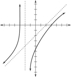
Turning Inside Out with Inverse Functions

Every operation in math has an inverse: addition undoes subtraction, multiplication undoes division (and vice versa for both). Because functions are just more complicated forms of operations, functions also have inverses. An inverse function simply undoes another function.

Perhaps the best reason to know whether functions are inverses of each other is that if you can graph the original function, you can usually graph the inverse as well. So that’s where we begin this section. At times in pre-calc you’ll be asked to show that two functions are inverses or to find the inverse of a given function, so you find that info later in this section as well.

If f(x) is the original function, f^–1(x) is the symbol for its inverse. This notation is used strictly to describe the inverse function and not

The negative is used only to represent the inverse, not the reciprocal.

Graphing an inverse

If you’re asked to graph the inverse of a function, you can do it the long way and find the inverse first (see the next section), or you can remember one fact and get the graph. What’s the one fact, you ask? Well, it’s that a function and its inverse are reflected over the line y = x. This line is a linear function that passes through the origin and has a slope of 1. When you’re asked to draw a function and its inverse, you may choose to draw this line in as a dotted line; this way, it acts like a big mirror, and you can literally see the points of the function reflecting over the line to become the inverse function points. Reflecting over that line switches the x and the yand gives you a graphical way to find the inverse without plotting tons of points.

The best way to understand this concept is to see it in action. For instance, just trust us for now when we tell you that these two functions are inverses of each other:

f(x) = 2x – 3

To see how x and y switch places, follow these steps:

1. Take a number (any that you want) and plug it into the first given function.

We picked –4. When f(–4), you get –11. As a point, this is written (–4, –11).

2. Take the value from Step 1 and plug it into the other function.

In this case, you need to find g(–11). When you do, you get –4 back again. As a point, this is (–11, –4). Whoa!

This works with any number and with any function: The point (a, b) in the function becomes the point (b, a) in its inverse. But don’t let that terminology fool you. Because they’re still points, you graph them the same way you’ve always been graphing points.

The entire domain and range swap places from a function to its inverse. For instance, knowing that just a few points from the given function f(x) = 2x – 3 include (–4, –11), (–2, –7), and (0, –3), you automatically know that the points on the inverse g(x) will be (–11, –4), (–7, –2), and (–3, 0).

So if you’re asked to graph a function and its inverse, all you have to do is graph the function and then switch all x and y values in each point to graph the inverse. Just look at all those values switching places from the f(x) function to its inverse g(x) (and back again), reflected over the line y = x.

You can now graph the function f(x) = 3x – 2 and its inverse without even knowing what its inverse is. Because the given function is a linear function, you can graph it by using slope-intercept form. First, graph y = x. The slope-intercept form gives you at least two points: the y-intercept at (0, –2) and moving the slope once at the point (1, 1). If you move the slope again, you get (2, 4). The inverse function, therefore, moves through (–2, 0), (1, 1), and (4, 2). Both the function and its inverse are shown in Figure 3-22.

Inverting a function to find its inverse

If you’re given a function and must find its inverse, first remind yourself that domain and range swap places in the functions. Literally, you exchange f(x) and x in the original equation. When you make that change, you call the new f(x) by its true name — f^–1(x) — and solve for this function.

For example, follow the steps to find the inverse of this function:

1. Switch f(x) and x.

When you switch f(x) and x, you get

You can also change f(x) to y and then switch x and y.

2. Change the new f(x) to its proper name — f^–1(x).

The equation then becomes

3. Solve for the inverse.

This step has three parts:

a. Multiply both sides by 3 to get 3x = 2f^–1(x) –1.

b. Add 1 to both sides to get 3x + 1 = 2f^–1(x).

c. Lastly, divide both sides by 2 to get your inverse:

Verifying an inverse

At times, your textbook or teacher may ask you to verify that two given functions are actually inverses of each other. To do this, you need to show that both f(g(x)) and g(f(x)) = x.

When you’re asked to find an inverse of a function (like in the previous section), we recommend that you verify on your own that what you did was correct, time permitting.

For example, show that the following functions are inverses of each other:

f(x) = 5x – 4

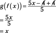
1. Show that f(g(x)) = x.

This step is a matter of plugging in all the components:

2. Show that g(f(x)) = x.

Again, plug in the numbers and start crossing out: