Two-Dimensional Calculus (2011)

Chapter 2. Differentiation

8. Level curves and the implicit function theorem

Let f(x, y) be continuously differentiable in a domain D and let (x₀, y₀) be any point in D. The equation f(x, y) = f(x₀, y₀) defines a level curve through the point (x₀, y₀). Let us assume for the moment that this level curve is the implicit form of a regular curve C, at least near (x₀, y₀). In other words, suppose we have a regular curve C: x(t), y(t), passing through (x₀, y₀), such that f(x, y) is constant on C. Using our earlier notation, this means

for some constant k. Then

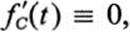
and by the chain rule, at the point t₀ corresponding to (x₀, y₀), we have

This equation may be interpreted in various ways. First, if the unit tangent to C at (x₀, y₀) is T_α = cos α, sin α , and if s is the parameter of arc length along C, we have

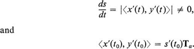
Thus we may write Eq. (8.1) as

and since s'(t₀) ≠ 0, we have

But the left-hand side of Eq. (8.3) is precisely ∇_αf(x₀, y₀). We are led to the following theorem.

Theorem 8.1 The directional derivative of a function at a point in the direction of a level curve through the point is always zero. The gradient of a function at a point is always orthogonal to the level curve through the point. (Both statements are made under the assumption that the level curve is a regular curve.)

PROOF. Both statements are immediate consequences of Eq. (8.3).

Example 8.1

Here the level curves x² + y² = k are circles about the origin; ∇f(x, y) = 2x, 2y is a vector in the direction of the radius to these circles at each point and is therefore orthogonal to the circle (Fig. 8.1).

The directional derivative of x² + y² in a direction tangent to the circle x² + y² = k is always zero.

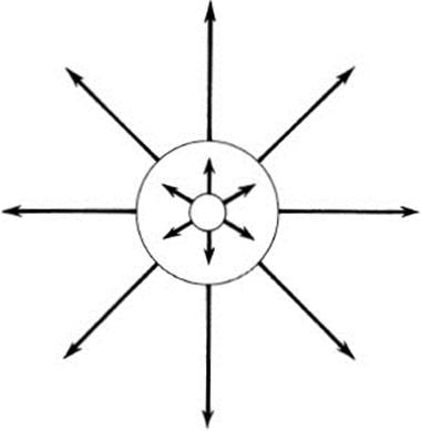
FIGURE 8.1 Level curves and gradient vectors for f(x, y) = x² + y²

Theorem 8.1 is based on the assumption that the equation f(x, y) = k actually represents a regular curve C, at least near a given point. Our main objective now is to prove that this is the typical case. In order to arrive at a general theorem, we consider first a special case. We ask when the equation f(x, y) = k can be solved in the form y = g(x), where g(x) is a differentiable function of x. If it can be solved, then we have

and by the chain rule

which is nothing but a special case of Eq. (8.1), where the parameter t is equal to x. From Eq. (8.4) it follows that if f_y ≠ 0,

Example 8.2

Find the slope of the curve

at the point (1, −1).

We let

Then

Thus,

The significance of Eq. (8.5) is that it allows us to compute the derivative of the function g(x) without actually knowing the function itself. In fact, there are extremely few cases where an equation f(x, y) = k can be solved explicitly in the form y = g(x). In Example 8.2, solving Eq. (8.6) for y as a function of x would be complicated, to say the least. Nevertheless, we can find the derivative of this function at any point on the curve.

One may well ask, what do we mean by “the function obtained by solving Eq. (8.6) for y in terms of x,” when we cannot in any practical sense solve Eq. (8.6) for y in terms of x. The answer to this question requires an understanding of the answer to the more basic question “what do we mean by a function?” For example, what do we mean by y = log₁₀ x? The answer is that we mean the number y such that 10^y = x. No explicit way for finding this number y need be given, but we must prove that for each x > 0 there is one and only one y such that 10^y = x in order to conclude that we have defined y as a function of x.

In the same way, if we wish to assert that Eq. (8.6) defines y as a function of x, at least near some point such as (1, −1), we have to show that for all values of x in some interval about x = 1, there is a corresponding value of ysatisfying Eq. (8.6). In this case it is easy to show that for any fixed value x₀, the equation

is satisfied by at least one value of y. (Namely, the left-hand side of this equation is a polynomial in y of odd degree, hence tends to +∞ as y → +∞ and tends to −∞ as y → −∞, and hence must be equal to 1 at some point.) The trouble here is that there may be several values of y satisfying this equation, and in order to obtain a well-defined function we must also restrict the interval in which y is allowed to lie (Fig. 8.2).

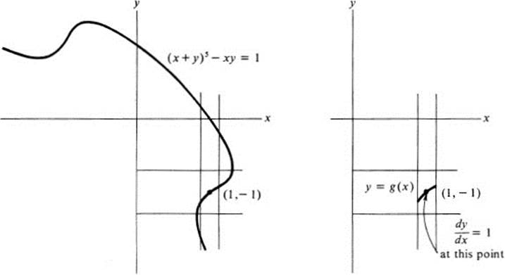
FIGURE 8.2 “Solving” (x + y)⁵ − xy = 1 in the form y − g(x) near (1, −1)

We may now make our earlier statements precise. When we say that

“Equation (8.6) can be solved in the form y = g(x) near the point (1, −1),”

we mean that

“there is some interval about x = 1, such that if we restrict y to an interval about y = −1, then Eq. (8.6) has one and only one solution for each fixed x.”

Alternatively, we may say that

“there exist positive numbers a, b such that for each x satisfying |x − 1| < a, there is exactly one solution of Eq. (8.6) satisfying |y + 1| < b.”

A final, more geometric, wording of the same statement, is that

“all points satisfying Eq. (8.6) and lying inside some rectangle |x − 1| < a, |y + 1| < b about the point (1, −1) lie on a curve y = g(x).”

We now state the general theorem which allows us to conclude that an equation f(x, y) = k can be solved in the form y = g(x). It is called the implicit function theorem, and an approximate form is: if f_y(x₀, y₀) ≠ 0, then the equation of the level curve f(x, y) = k passing through (x₀, y₀) can be solved in the form y = g(x) near (x₀, y₀).

Theorem 8.2 Implicit Function Theorem Let f(x, y) be continuously differentiable in D. Let (x₀, y₀) be any point in D such that

Then there exist numbers δ > 0 and > 0, and there exists a continuously differentiable function g(x) defined for |x − x₀| ≤ δ such that if |x − x₀| ≤ δ and |y − y₀| ≤ , then

PROOF. The proof falls into two completely separate parts. The first part shows that there exists a function g(x) satisfying Eq. (8.8). By its definition, this function need not even be continuous. In the second part we show that anyfunction g(x) satisfying Eq. (8.8) must in fact be continuously differentiable if f(x, y) is.

Part I. Existence of g(x) Let f_y(x₀, y₀) = η Our basic assumption is that η ≠ 0. We may assume η > 0. (If η < 0 apply the reasoning below to the function −f.) Then, by the continuity of f_y, we have for r sufficiently small,

if

This means that inside this circle f is a strictly increasing function of y for each fixed x. In particular, if we choose any positive number < r, we have

By the continuity of f(x, y), we can vary x₀ slightly on the left- and right-hand sides of (8.10), and the inequality still holds. More precisely, we can choose δ > 0 so that

If δ is sufficiently small, then the rectangle

lies inside the circle, so that Eq. (8.9) still holds in this rectangle (Fig. 8.3). Equation (8.11) asserts that along the bottom of this rectangle f(x, y) < f(x₀, y₀), while on the top f(x, y) < f(x₀, y₀). Thus on each vertical line segment x = x₁the function f(x₁, y) must pass through the value f(x₀, y₀) at some point (x₁, y₁) (Fig. 8.4). Further, there is only one such point on each vertical segment, since by (8.9), f(x₁, y) is a strictly increasing function of y. We set g(x₁) equal to this unique number y₁. This defines the function g(x) for |x − x₀| < δ in such a way that Eq. (8.8) holds.

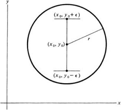
FIGURE 8.3 A neighborhood of (x₀, y₀) in which f_y(x, y) ≥ η/2 > 0

Part II. Smoothness of g(x) The fact that the function g(x) is continuously differentiable does not depend on the particular way in which we defined it, but is a general property, which may be stated roughly as follows: the level curves of a smooth function are smooth curves. We give this statement precise form in the following “regularity lemma.”

Lemma 8.1 If f(x, y) is continuously differentiable in D and satisfies (8.7), then any function g(x) satisfying (8.8) must be continuously differentiable.

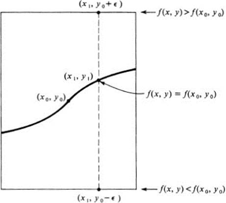
FIGURE 8.4 Existence of y₁ such that f(x₁, y₁) = f(x₀, y₀)

PROOF. Define the numbers δ and as in part I of the proof of Th. 8.2. We consider any two values x₁, x₂ in |x − x₀| < δ, and let

Then, by (8.8),

The mean-value theorem (Th. 7.3) tells us that there is a point (x₃, y₃) on the line segment from (x₁, y₁) to (x₂, y₂) such that

But by (8.14), the left-hand side of Eq. (8.15) is zero, and hence

whence

by (8.9). But f_x is continuous in the rectangle defined by (8.12), and hence |f_x| has a maximum M there. Thus

Hence x₂ → x₁ ⇒ y₂ → y₁ ⇒ g(x₂) → g(x₁), by (8.13). This means precisely that g(x) is continuous at x₁. Since (x₃, y₃) is on the line segment between (x₁, y₁) and (x₂, y₂), we have further that x₂ → x₁ ⇒ x₃ → x₁ and y₃ → y₁. From Eq. (8.16), we conclude that

Thus the limit on the left-hand side exists, and it is by definition (using Eq. (8.13) ), g'(x₁). Explicitly,

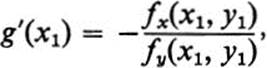
where y₁ = g(x₁). Since x₁ was any value of x in |x − x₀| < δ, we have

Thus g(x) is differentiable in |x − x₀| < δ, and since the right-hand side of Eq. (8.17) is a continuous function of x, g'(x) is continuous in |x − x₀| < δ. This concludes the proof of the lemma, and hence of the theorem.

Remark. In the course of this proof we have used several basic properties of continuous functions. They are the following.

1. If f(x) is continuous for a ≤ x ≤ b, and if f(a) = c, f(b) = d, then given any number y₀ between c and d, there is some x₀ between a and b such that f(x₀) = y₀. Geometrically, this means that the graph of a continuous function intersects every horizontal line between its initial and terminal values (Fig. 8.5). This is called the “intermediate-value property” of continuous functions, and is often used (even if not explicitly stated) in calculus. To prove it requires a careful study of the real number system.³

2. If f(x, y) is continuous at (x₀, y₀), and if f(x₀, y₀) = η > 0, then for some r > 0, f(x, y) ≥ η/2 in the whole circle (x − x₀)² + (y − y₀)² > r². This is an elementary fact that follows directly from the definition of continuity (see Ex. 5.16a).

3. If f(x, y) is continuous in a rectangle |x − x₀| ≤ δ, |y − y₀| ≤ then it is bounded; that is, for some fixed M, |f(x, y)| ≤ M in the whole rectangle. The proof of this again entails a fundamental study of the real number system. We actually stated a somewhat stronger result; namely that f(x, y) has a maximum in the rectangle. This means that f(x, y) ≤ M in the

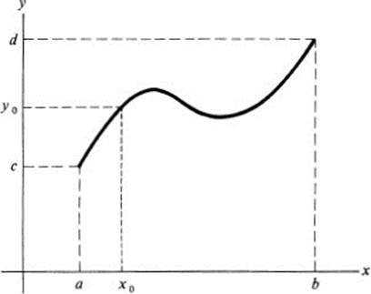
FIGURE 8.5 Intermediate-value property of continuous functions

whole rectangle, and further that f(x₁, y₁) = M for some point (x₁, y₁) in the rectangle.

For the sake of completeness we state (without proof) a general theorem of which the statements in paragraph 3 are special cases. We need first two definitions.

Definition 8.1 A set S of points in the plane is bounded if it lies inside some circle x² + y² < r².

Definition 8.2 A set S of points in the plane is closed if it contains all its boundary points.

Example 8.3

If P₁(x, y),…, P_r(x, y) are polynomials (or any functions continuous in the whole plane), then the set of points satisfying all of the inequalities

is a closed set. Thus, a disk x² + y² ≤ 1 and a rectangle |x − x₀| ≤ δ, |y − y₀| ≤ are examples of closed, bounded sets.

Theorem 8.3 If f(x, y) is continuous on a closed, bounded set S, then it has a maximum M at some point of S.⁴

Returning to Th. 8.2, we see that if the roles of x and y are reversed and if f_x(x₀, y₀) ≠ 0, then the equation f(x, y) = f(x₀, y₀) can be solved near (x₀, y₀) in the form x = h(y).

Corollary Let f(x, y) be continuously differentiable in D and suppose ∇f(x₀, y₀) ≠ 0. Then near (x₀, y₀), the level curve f(x, y) = f(x₀, y₀) defines a regular curve x(t), y(t).

PROOF. Since ∇f(x₀ y₀) ≠ 0, we have either f_y(x₀, y₀) ≠ 0 or f_x(x₀, y₀) ≠ 0 (or both). In the first case we can solve f(x, y) = f(x₀, y₀) in the form y = g(x), which gives a regular curve with x = t. In the second case we may write x = h(y), which is a regular curve with y = t.

Geometrically, we may picture the situation as follows. A point where ∇f ≠ 0, defines a point on the side of the mountain z = f(x, y). At such a point, the intersection of z = f(x, y) with a horizontal plane z = f(x₀, y₀), yields a smooth contour line (Fig. 8.6). Somewhat less picturesquely, the condition ∇f ≠ 0 means precisely that the tangent plane to the surface z = f(x, y) at the point is not horizontal.

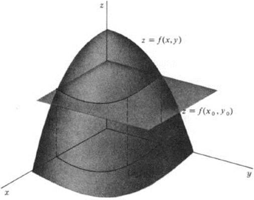
FIGURE 8.6 Geometric interpretation of the implicit-function theorem

Example 8.4

Hence ∇f = 0 only at the origin. The level curve through any other point is a regular curve. The “level curve” x² + y² = 0 consists of the single point (0, 0).

Example 8.5

Again ∇f = 0 only at the origin. The “level curve” xy = 0 through the origin consists of the entire x and y axes. Since these cross at the origin, they clearly do not form a regular curve in any circle about the origin.

Example 8.6

Here,

Since cos y ≥ −1 for every y, we have

at every point. Hence ∇f is never zero, and the level curves of this function are regular curves near every point. In fact, f_y > 0 everywhere, and hence the equation f(x, y) = c can be solved in the form y = g(x) near each point.

Exercises

8.1 Find the slope of the curve (x + y)⁵ − xy = 1 at the following points:

a. (1,0)

b. (0, 1)

c. (1, −2)

d. (−2,1)

e. the point on the curve where y = x

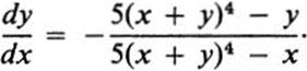
8.2 Assume that each of the following equations can be solved in the form y = g(x). and use Eq. (8.5) to find dy/dx.

a. x sin y − y cos x = 0

b. x + 2y² + sin xy = 1

c. x³ − 2xy + y² = 5

d. xe^y − y² + x = 0

Note: in practice, it is often easier to use the method that led to Eq. (8.5) rather than Eq. (8.5) itself. In other words, given an equation that defines y implicitly as a function of x, consider y replaced by that function so that the equation becomes an identity in x, and then differentiate with respect to x, using the rule for composite functions of one variable. For example, differentiating

yields

and solving for dy/dx, we obtain

8.3 Find dy/dx for each of the equations in Ex. 8.2 by the method just indicated.

8.4 For each of the following equations, find dy/dx by the implicit function method of Exs. 8.2 or 8.3. Then solve explicitly for y as a function of x and differentiate. Check that your answer is the same in both cases.

a.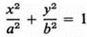

b. ye^x − x² + y = 0

c. e^x + e^y + e^{x + y} = 1

d. x + xy + y = 1

Note: an advantage of the implicit function method for finding the derivative dy/dx, even in the cases where it is possible to solve explicitly for y as a function of x, is that the computations are often simpler. A disadvantage is that the answer is expressed in terms of both x and y. It is still possible to take higher derivatives by using the same method. The original equation can often be used at various stages along the way to simplify the expressions obtained. For example, if x² + y² = 1, then

Hence,

8.5 Use the above method of implicit differentiation to find d²y/dx² for each of the equations in Ex. 8.4.

8.6 Show that if ∇f(x₀, y₀) ≠ 0, then the equation of the tangent line to the level curve f(x, y) = f(x₀, y₀) at the point (x₀, y₀) is

*8.7 Show that all level curves of the function

intersect all rays through the origin at an angle of 45°. (Hint: Show that if (x₀, y₀) is any point on a level curve f(x, y) = c, tan α is the slope of the curve at that point, and tan θ = y₀/x₀, then tan α = tan (θ + π).)

8.8 Explain Exs. 6.5 and 6.6 in the light of Th. 8.1.

8.9 For each of the functions of Ex. 6.3, sketch the level curve through the point (1, 1) and verify Th. 8.1.

8.10 If f(x, y) = sin log cosh tan e^{x2 + y2}, find f_x(0, 1). (Hint: do not calculate. Think!)

8.11 For each of the following pairs of functions f(x, y), g(x, y) show that each level curve of f(x, y) intersects at right angles all level curves of g(x, y). (More precisely, this property holds at all points of intersection where both level curves are regular curves.)

a. f(x, y) = x² − y², g(x, y) = xy

b. f(x, y) = x² + y², g(x, y) = y²/x²

c. f(x, y) = e^x cos y, g(x, y) = e^x sin y

8.12 a. Write an equation involving the partial derivatives of f(x, y) and g(x, y) that is equivalent to the condition that the level curves of f and g intersect at right angles wherever f and g have nonzero gradient.

b. Show that any pair of functions satisfying the Cauchy-Riemann equations f_x = g_y, f_y = − g_x, have the property that their level curves intersect at right angles.

c. Show that the converse of part b is false.

8.13 An important quantity in meteorology is atmospheric pressure. When the atmospheric pressure is considered as a function of position over a portion of the earth’s surface, the level curves are called isobars. In the absence of other forces, the gradient of this function would indicate the magnitude and direction of winds. The air would tend to travel from higher to lower pressure areas, the speed would be proportional to the rate of change of pressure and the direction would be that of the maximum rate of change of pressure. Thus, by Th. 8.1, the direction of winds would be perpendicular to the isobars. In fact, other factors, such as the rotation of the earth, deflect the winds, but a map showing the isobars is still a basic component for predicting winds and weather in general. (See Fig. 8.7 where atmospheric pressure is given in inches of mercury (29.2 to 30.6) and in millibars (989 to 1036).)

Explain why the wind velocity tends to be small near the center of either a high pressure or a low pressure area. (The “doldrums” are the low-pressure areas near the equator, and the “horse latitudes” refer to the high-pressure belts over the oceans at around 30° latitude North and South of the equator.)

8.14 For each of the following functions f(x, y) and points (x₀, y₀), check whether the condition f_y(x₀, y₀) ≠ 0 is satisfied. If not, decide whether the conclusion of Th. 8.2 is valid, and if it is not explain what part of it fails.

a. f(x, y) = x² + y², (x₀, y₀) = (−5, 0)

b. f(x, y) = x² + y², (x₀, y₀) = (−4, 3)

c. f(x, y) = x + y³, (x₀, y₀) = (0, 0)

d. f(x, y) = x² + 2xy + y², (x₀, y₀) = (0, 0)

8.15 Show that the equation (x + y)⁵ − xy = 1 defines a regular curve near each of its points. (Hint: show that a simultaneous solution of f_x = 0 and f_y = 0 cannot lie on the curve.)

8.16 For each of the following functions f(x, y), sketch and describe in words the level curve f(x, y) = 0. Check in particular any points on the curve where ∇f = 0, and describe the curve near those points.

a. f(x, y) = x² − y³

b. f(x, y) = x⁴ + y⁴

c. f(x, y) = x² + y² − 1)(x² + y²)

d. f(x, y) = x² + y² − 1)²

e. f(x, y) = x² + y² + e^xy

*f. f(x, y) = x³ − x² + xy² + y²

(Hint: in part f, either solve for y as a function of x, or else use the parametric form given in Ex. 2.13.)

8.17 The inverse function theorem for functions of one variable may be stated as follows. If h(y) is differentiable and h'(y₀) ≠ 0, then the equation x = h(y)

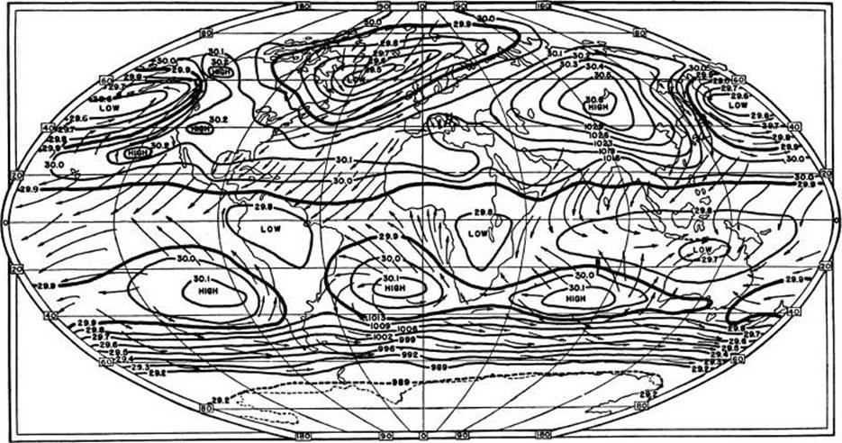
FIGURE 8.7 Mean January sea-level pressures and wind directions of the world [Thomas A. Blair and Robert C. Fite, Weather Elements, 4th Ed., © 1957. Reprinted by permission of Prentice-Hall, Inc., Englewood Cliffs, New Jersey. Base map Copyright Denoyer-Geppert Company, Chicago, used by permission.]

can be solved near x₀ = h(y₀) in the form y = g(x), where g(x) is differentiable and g'(x₀) = 1/h'(y₀). By considering the function f(x, y) = h(y) x, show how this theorem is related to the implicit function theorem, Th. 8.2.

8.18 Kepler’s laws of planetary motion (see Ex. 7.25) do not give the position of a planet explicitly as a function of time. However, if a planet moves along the ellipse x = a cos φ, y = b sin φ, where the sun is at the focus (c, 0), and if t is the time from the moment the planet passes the point (a, 0) (the perihelion) to the position corresponding to a given value of φ, then it follows from Kepler’s second law that φ and t are related by Kepler’s equation

where k is a positive constant. (We are using the standard notation for an ellipse: c = (a² − b²)^1/2, = c/a. Thus, 0 < < 1.)

a. Show that for an arbitrary pair of values t₀, φ₀ satisfying Kepler’s equation, there exists a solution of that equation in the form φ = g(t) near (t₀, φ₀).

b. Show that if g(t) is the function of part a, then

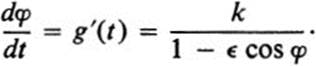
c. Deduce that dφ/dt is maximum at perihelion (a, 0), and minimum at aphelion (− a, 0).

d. Find the velocity vector v(t) = x'(t), y'(t) at an arbitrary point.

*e. Show that the speed |v(f)| decreases continually from perihelion to aphelion, and then increases from aphelion to perihelion. (Hint: express |v(t)|² as a function of cos φ. Call this function f(u), where u = cos φ. Show that f'(u) > 0 for all u, so that f(u) increases when u increases and decreases when u decreases.)