Two-Dimensional Calculus (2011)

Chapter 2. Differentiation

11. Higher order derivatives

If f(x, y) is continuously differentiable, then f_x and f_y are by definition continuous functions of x and y. We may ask whether they in turn are differentiable. If so, we may form (f_x)_x, (f_x)_y, etc. We adopt the following notation:

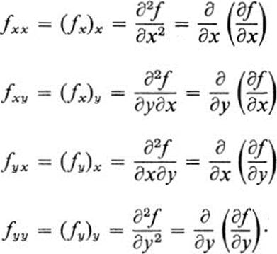
These are called the second-order partial derivatives of f(x, y).

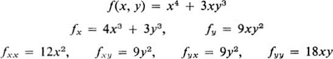
Example 11.1

Example 11.2

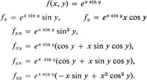
The equality of the so-called “mixed partial derivatives” f_xy and f_yx in the first example might pass for a coincidence, but it seems improbable in the second example unless there is a general rule. Indeed there is, and it is the following.

Theorem 11.1 If f_xy and f_yx exist and are continuous, then they are equal.

PROOF. Choose any point (x₀, y₀), and assume that the hypotheses of the theorem are satisfied inside some circle about (x₀, y₀). Let (x₁, y₁) be any other point in this circle, and form the function (see Fig. 11.1)

By the mean-value theorem there is a y₂ between y₀ and y₁ such that

But by Eq. (11.1),

where the second equality is obtained by applying the mean-value theorem to the function f_y(x, y₂). Combining Eqs. (11.1), (11.2), and (11.3) yields

where (x₂, y₂) is some point in the rectangle indicated in Fig. 11.1.

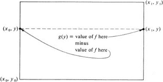
FIGURE 11.1 Notation for proof that f_xy = f_yx

The same reasoning applied to the function

yields

and

whence

where (x₃, y₃) is again a point in the same rectangle.

Comparing Eqs. (11.4) and (11.5), we see that

Finally, as (x₁, y₁) → (x₀, y₀) we have (x₂, y₂) → (x₀, y₀) and (x₃, y₃) → (x₀, y₀), so that the continuity of f_xy and f_yx applied to Eq. (11.6) yields f_yx(x₀, y₀) = f_xy(x₀, y₀), which proves the theorem.

Remark Lest it be thought that equality of f_xy and f_yx is too obvious to need a proof, we give the following example.

Let

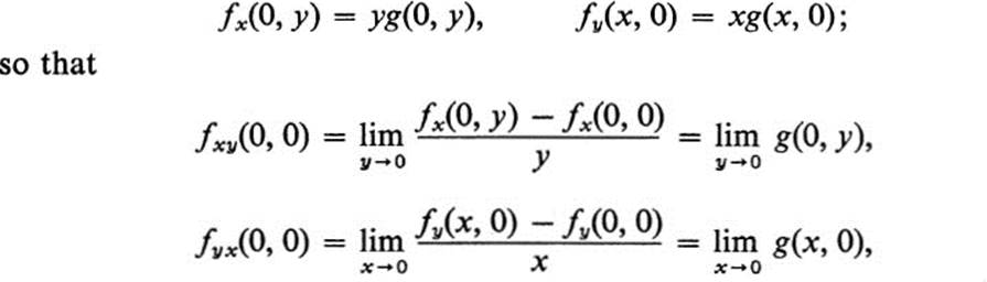
where g(x, y) is defined and differentiable everywhere except at the origin. We shall see how to choose g(x, y) so that f_xy ≠ f_yx. First we note that f ≡ 0 on the x and y axes so that f_x(0, 0) = f_y(0, 0) = 0. Next, if (x, y) ≠ (0, 0), we have

In particular,

and the question reduces to the equality of these two limits. Now if g(x, y) is continuous at the origin, then both limits are the same and equal g(0, 0). However, a simple choice, such as

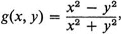
yields

and

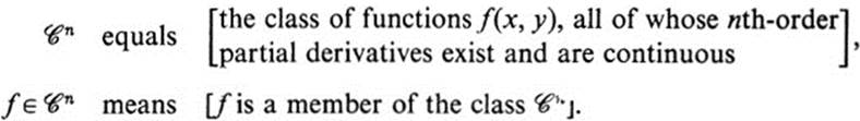
In the example that we have just given, the partial derivatives f_xy and f_yx exist everywhere, but they are not continuous at the origin, and hence Theorem 11.1 does not apply. The case where some derivative exists but is not continuous may be considered exceptional. In most problems, either derivatives of all orders exist and are continuous, as in the case of polynomials, trigonometric functions, and exponential functions, or else some derivative fails to exist, as in the case of fractional exponents. It is convenient to introduce the notation

meaning f is continuously differentiable, and

meaning all second-order derivatives of f exist and are continuous. Thus, if f , Th. 11.1 applies, and f_xy = f_yx, so that f has essentially three distinct second-order derivatives f_xx, f_xy, f_yy.

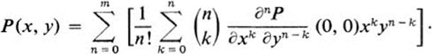
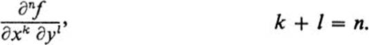
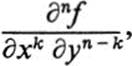
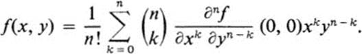
In a similar manner we can form higher order derivatives, where an nth-order partial derivative is obtained by n successive differentiations, each with respect to either x or y. We introduce the notation

Now if f , then all the (n − 1)-order partial derivatives of f are continuously differentiable, hence continuous, and therefore f . Thus, the classes are each included in the previous ones:

where the notation denotes the class of continuous functions. Furthermore, we have

Applying Th. 11.1, which allows interchanging the order of differentiation at each step, we come to the following conclusion.

If f , then the nth-order partial derivatives do not depend on the order of differentiation, but only on the total number of times f is differentiated with respect to x and y. If f is differentiated k times with respect to x and l times with respect to y, we obtain an nth-order derivative if k + l = n. The notation for this is

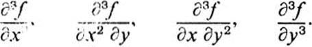
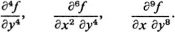
Thus the third derivatives of f(x, y) are

In general, a function f(x, y) has n + 1 distinct nth-order derivatives

k = 0, 1, 2,…, n.

Example 11.3

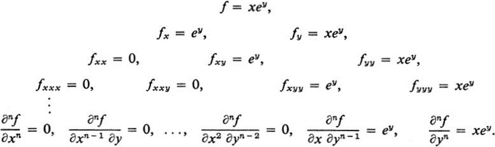
Thus, for this particular function, partial differentiation any number of times with respect to the variable y leaves the function unchanged; all derivatives involving one differentiation with respect to x and the rest with respect to y are equal to e^y; and all derivatives involving two or more differentiations with respect to x are equal to zero.

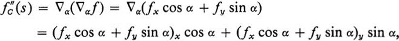
Higher Order Directional Derivatives

The meaning of the second-order partial derivatives f_xx(x₀, y₀), and f_yy(x₀, y₀) is quite clear, since they are the ordinary second derivatives of the functions f(x, y₀) and f(x₀, y), respectively. The necessity for considering the quantity f_xy becomes clear if we try to compute the ordinary second-derivative of f with respect to arc length along an arbitrary straight line through (x₀, y₀). If we let

denote such a line, and use again the notation

then

We now introduce the notation

wherever the derivatives on the right exist. Thus, the nth-order directional derivative of f in the direction α is the ordinary nth-order derivative of f with respect to arc length along the straight line in the direction α.

Suppose now that f . Then

and since the right-hand side is continuously differentiable, we have

or

The importance of this formula is that it allows us to describe very accurately how the surface z = f(x, y) behaves near any given point (x₀, y₀). We need only observe that if the left-hand side, (x₀, y₀), is positive, then > 0, so that the curve on the surface lying over the straight line C is concave upwards (Fig. 11.2). Similarly, < 0 means that this curve is concave downwards. Suppose now that we fix (x₀, y₀) and set

Then a, b, c are constants, and as α varies from 0 to 2π, (x, y) goes once around the circle X² + Y² = 1. Equation (11.7) becomes

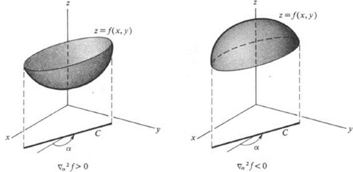
FIGURE 11.2 Geometric interpretation of the sign of the second directional derivative

and we see that the totality of .values of (x₀, y₀) is precisely the set of values of a quadratic form on the unit circle. We may apply all the results of the previous section to describe the behavior of the surface z = f(x, y). For example, if the quadratic form is positive definite, then over each straight line the surface will be convex upwards, while if it is negative definite, the surface will be convex downwards (Fig. 11.3). If the quadratic form takes on both positive and negative values, then the surface will be convex upwards over certain lines through (x₀, y₀) and convex downwards over others. Such a point is called a saddle point (Fig. 11.4).

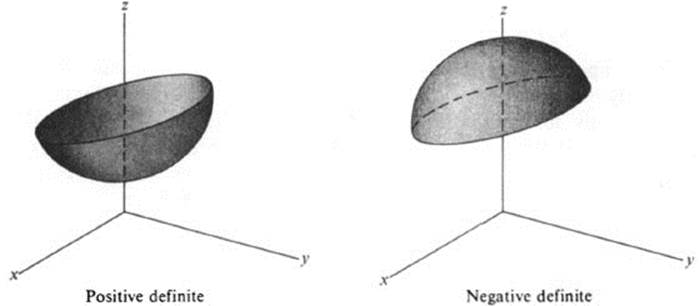
FIGURE 11.3 Picture of surfaces whose second directional derivatives are positive definite or negative definite

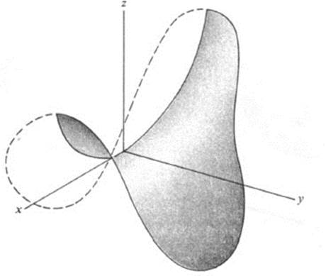
FIGURE 11.4 Saddle surface

Example 11.4

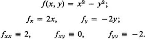
This surface is concave up in the x direction and concave down in the y direction. Every point is a saddle point.

We shall discuss these cases in more detail in the next section, and also their use in maximum-minimum problems. We give now just one illustration of this line of reasoning.

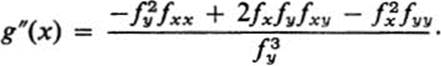
Theorem 11.2 Suppose f(x, y) and

Then f(x, y) can have neither a local maximum nor a local minimum at (x₀, y₀).

Remark This is a result that has no analog for functions of a single variable, since there is no condition analogous to (11.10).

PROOF. Condition (11.10) is precisely the condition ac − b² < 0 that guarantees that the quadratic form (11.9) takes on both positive and negative values. In other words, there are a pair of lines C₁, C₂ through (x₀, y₀) such that for the corresponding directions α₁, α₂ we have Thus, and But from the theory of functions of a single variable, this means that cannot have a local maximum and cannot have a local minimum. But if f(x, y) had a local maximum or minimum at (x₀, y₀), then the same would be true of both and , which are merely restrictions of f to straight lines. Hence f can have neither, and the theorem is proved.

Remark Condition (11.10) means geometrically that (x₀, y₀) is a saddle point, so that the theorem is intuitively obvious.

Example 11.5

Here

This function cannot have a local maximum or minimum anywhere.

Example 11.6

f(x, y) is a harmonic function. This means that f(x, y) satisfies the equation

This equation is met in many areas of mathematics and its applications, and the study of its solutions has led to a theory, known as potential theory. We note that from Eq. (11.11) we have f_xx = −f_yy, and hence

everywhere, with equality possible only if

We have the following basic property: a harmonic function cannot have a local maximum or minimum unless it is constant. In fact, by what we have just observed, either

in which case f cannot have a local maximum or minimum by Th. 11.2 or else

in which case all the second-partial derivatives are zero. We can also show in this case that f cannot have a local maximum or minimum unless all higher derivatives vanish too, in which case f is constant.⁷ Examples of harmonic functions include all constants, all linear functions, and the quadratic function given in Example 11.5.

We conclude this section with the observation that Eq. (11.7) may be extended by induction to the general formula

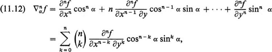
where is the binomial coefficient,

Exercises

11.1 Find all second-order partial derivatives of the following functions.

a. f(x, y) = x⁶ − 5x⁴y² + 3xy⁵

b. f(x, y) = e^x + log y

c. f(x, y) = sin (y/x)

d. f(x, y) = tan (x + y)

e. f(x, y) = (x − y)⁵

f.

11.2 Show that each of the following functions f(x, y) is harmonic, that is, f_xx + f_yy ≡ 0.

a. f(x, y) = xy

b. f(x, y) = x³ − 3xy²

c. f(x, y) = x/(x² + y²)

d. f(x, y) = sin x cosh y

11.3 Suppose that the functions f(x, y), g(x, y) satisfy the Cauchy-Riemann equations

Show that if f(x, y) and g(x, y) , then f(x, y) and g(x, y) are both harmonic.

11.4 Verify the statement of Ex. 11.3 for the following pairs of functions.

a. f(x, y) = x² − y², g(x, y) = 2xy

b. f(x, y) = e^x cos y, g(x, y) = e^x sin y

c.

11.5 a. Show that a quadratic form is a harmonic function if and only if it can be expressed as a(x² − y²) + 2bxy, where a and b are arbitrary constants.

b. Show that if f(x, y) and f(x, y) is harmonic, then

are harmonic also.

Note: in Exs. 11.6–11.9 assume that all functions are at least twice continuously differentiable.

11.6 Let f(x, y) = g(x) + h(y).

a. Show that f_xy ≡ 0.

b. Show that if g″(x) > 0 and h″(y) < 0, then the surface z = f(x, y) cannot have a local maximum or minimum at any point.

c. Verify parts a and b for the function of Ex. 11.1b.

11.7 a. Show that the functions in Exs. 11.1d, e, f, satisfy f_xx − f_yy ≡ 0.

b. Show that any function of the form

satisfies the equation f_xx − f_yy = 0.

11.8 Suppose that f(x, y) = g(x² + y²).

a. Find f_xx, f_xy, and f_yy in terms of the function g and its derivatives.

*b. Show that if f(x, y) is a harmonic function that depends only on the distance r of the point (x, y) to the origin, then

where c and d are constants. (Hint: write f(x, y) in the form g(x² + y²). Using part a, show that, with t = x² + y², g(t) satisfies the equation

11.9 Let f(x, y) be homogeneous of degree k.

a. Show that f(x, y) satisfies the equations

b. Show that f(x, y) satisfies

11.10 Verify the equation in Ex. 11.9b for the functions of Exs. 11.1a, c, e.

11.11 Let f(x, y) = e^x sin y.

a. Find all third-order derivatives of f(x, y).

b. Find

c. Find

d. Given any two integers k and l, with k + l = n, describe how ∂ⁿf/∂x^k ∂y^l depends on k and l.

11.12 Let f(x, y) = e^xy.

a. Find all fourth-order derivatives of f(x, y).

b. What is ∂^kf/∂x^k?

c. What is ∂^{k + 1}f/∂x^k ∂y?

d. What is ∂^{k + 1}f/∂x ∂y^k?

*e. What is the value at the origin of ∂^{k + 1}f/∂x^k ∂y^l, for arbitrary k and l?

11.13 Let f(x, y) = 3x² − 8xy + 2y² + 12x − 4y + 17.

a. Find for arbitrary α.

b. Find an α such that > 0.

c. Find an α such that < 0.

d. Can f(x, y) have a local maximum or minimum at any point?

11.14 Let f(x, y) = ax² + 2bxy + cy² + dx + ey + f, where a and c have opposite signs.

a. By examining the function on any pair of lines x = x₀ and y = y₀, show that it is concave upwards in one case and downwards in the other, so that f(x, y) cannot have a local maximum or minimum at (x₀, y₀).

b. Use Th. 11.2 to derive the same conclusion.

11.15 Let f(x, y) = log [1/(3x + 7xy + 2y + 1)].

a. Find

b. For which values of α is (0, 0) > 0?

11.16 Let f(x, y) = exp { [7x² + 10xy + 7y²]}. Find the maximum and minimum of (0, 0) for 0 ≤ α ≤ 2π.

11.17 Given f_c(t) = f(x(t), y(t)), find .

11.18 Explain why the terms involving f_x and f_y in the answer to Ex. 11.17 do not appear in Eq. (11.7).

11.19 Let r = (x² + y²)^1/2.

a. Find r_xx, r_xy, r_yy.

b. If x and y are functions of t, find d²r/dt², first by using the answer to Ex. 11.17, and then by direct differentiation.

c. If is considered as a quadratic form in the variables X = cos α, Y = sin α, classify it according to the categories of the previous section, that is, positive definite, positive semidefinite, etc.

d. Sketch the surface z = (x² + y²)^1/2, and interpret geometrically your answer to part c.

11.20 Let z = (1 − x² − y²)^1/2, for x² + y² < 1.

a. Find z_xx, z_xy, z_yy.

b. Answer Ex. 11.19c for this function.

c. Answer Ex. 11.19d for this function.

*11.21 a. Suppose the equation f(x, y) = c satisfies the assumptions of the implicit function theorem and defines a curve y = g(x). Show that if f(x, y) , then g(x) is twice continuously differentiable and

b. Using the formula

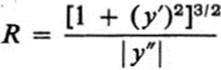
for the radius of curvature of a curve y = g(x), where y″ ≠ 0, find a formula for the radius of curvature of a curve in the implicit form f(x, y) = c.

c. Apply the formula of part b to find the radius of curvature at an arbitrary point of the circle x² + y² = r².

11.22 a. Find the expression for by taking the directional derivative ∇_α of the right-side of Eq. (11.7).

b. Find by substituting n = 3 in Eq. (11.12), and compare the result with your answer to part a.

11.23 Carry out Ex. 11.22a, b for .

*11.24 Prove Eq. (11.12) by induction.

*11.25 Show that the function f(x, y) = x³ + x²y − 2xy² + y³ cannot have a local maximum or a local minimum at any point.

11.26 a. If f(x, y) = cxⁱy^j, find ∂^kf/∂x^k.

b. If f(x, y) = cxⁱy^j, find ∂^{k + l}f/∂x^k ∂y^l.

c. If f(x, y) = cxⁱy^j, find the value of ∂^{k + l}f/∂x^k ∂y¹ at (0, 0).

d. If

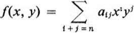
is a homogeneous polynomial of degree n, find (∂^mf/∂x^k ∂y^l)(0, 0), where k + l = m.

e. Show that the homogeneous polynomial f(x, y) of part d may be written in the form

f. Show that an arbitrary polynomial P(x, y) of degree m may be written in the form