Two-Dimensional Calculus (2011)
Chapter 4. Integration
21. Line integrals
In our study of functions of two variables, we used the technique of restricting a function to an arbitrary curve, thus obtaining a function of a single variable. Given a function f(x, y) defined at every point of a curve
![]()
we used the notation
![]()
for the function of one variable obtained in this way.
We adopt a parallel method in our study of integration of functions of two variables and introduce so-called line integrals. There are a number of possibilities concerning the variable with respect to which we integrate. We start with the following definition.
Definition 21.1 Let f(x,y) be a function that is defined and continuous at every point of a differentiable curve (21.1). We define ∫c f dx and ∫cf dy by
![]()
![]()
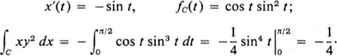
Example 21.1
If f(x, y) = xy2, find ∫c f dx for
![]()
We have
Example 21.2
if f(x, y) = xy2, find ∫c f dx for
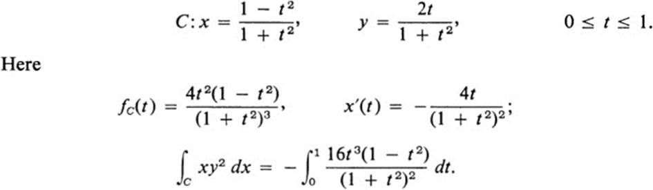
The answer is thus expressed as an ordinary integral of a rational function. We do not carry out the computation, since we shall find the value of this integral by a different reasoning a little later on.
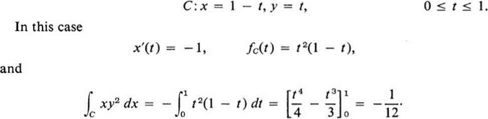
Example 21.3
If f(x, y) = xy2, find ∫c f dx for
As in Examples 21.1-21.3 we are interested in the way a line integral for a given function f depends on the choice of the curve C. The first important observation may be stated roughly as follows: the values of the line integrals (21.3) and (21.4) do not depend on the choice of the parameter t used to describe the curve C. More precisely, we have the following statement.1
Lemma 21.1 Let C be a differentiable curve defined by (21.1). Let h(τ) ∈![]() for α ≤ τ ≤ β, where a ≤ h(τ) ≤ b, and h(α) = a, h(ß) = b. Consider the curve obtained from C by setting t = h(τ);
for α ≤ τ ≤ β, where a ≤ h(τ) ≤ b, and h(α) = a, h(ß) = b. Consider the curve obtained from C by setting t = h(τ);
![]()
(Fig.21.1). Then for any continuous function f(x,y),

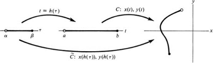
FIGURE 21.1Change of parameter defining a curve
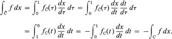
PROOF. We have

the first and last in this line of equalities are statements of the definition (21.3) of the line integral. The second equality is an application of the chain rule to the function x(h(τ)), and the third follows from the rule for change of variables in integration,
![]()
this rule being applied to the function g(t) = fc(t)dx/dt. Thus the first equation in (21.6) is verified. The second follows in the same manner. ![]()
Corollary When expressing a line integral, Eqs. (21.3) or (21.4), we may assume that the parameter for the curve C varies over the interval from 0 to 1.
PROOF. Given an arbitrary curve C of the form (21.1), we may set t = a + (b − a)τ, 0 ≤ τ ≤ 1, and we obtain the same values for the line integrals (21.3) and (21.4) using the parameter τ. ![]()
Let us now reconsider Examples 21.1 and 21.2. In Example 21.1, the curve C consists of the arc of the unit circle lying in the first quadrant, starting at (1,0) and ending at (0, 1) (Fig. 21.2). In Example 21.2, we may confirm by a direct computation that x(t)2 + y(t)2 ≡ 1, so that the curve C lies on the unit circle. Furthermore, we see that y ≥ 0 throughout, while x decreases from 1 to 0 as t goes from 0 to 1.Thus the curve C describes the same arc of the unit circle in the same direction as in Example 21.1. Since the parameter in Example 21.1 represents the polar angle at the origin, if we denote that angle by τ, itis clear that the parameter t in Example 21.2 should be expressible as a function of τ. In fact, setting t = tan (τ/2) in the curve C of Example 21.2 yields x = cos τ, y = sin τ, and by Lemma 21.1 the value of the line integral is the same as in Example 21.1.
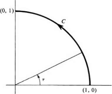
FIGURE 21.2Circular arc: x = cos τ, y = sin τ, 0 ≤ τ ≤ ![]()
It is important to observe that a curve defined parametrically in the form(21.1) has a natural direction or orientation, namely the direction associated with increasing values of the parameter t. Thus the initial point on the curve is the point x(a), y(a), and the endpoint is x(b), y(b). The changes of parameter allowed in Lemma 21.1 preserved the orientation, since we required that h(α) = a, h(β) = b. If we choose a parameter that reverses the sense in which the curve is described, then the line integral changes sign. To see this, we may assume by the Corollary to Lemma 21.1 that the parameter describes the interval from 0 to 1. We may then state the result as follows.
Lemma 21.2 Let C be a differentiable curve of the form
![]()
Let ![]() be the curve obtained from C by setting
be the curve obtained from C by setting
![]()
Then for any continuous function f(x, y),

PROOF. Just as in the proof of Lemma 21.1, we have
The only difference is that when applying the rule for changing the variable of integration, we must be careful to insert the correct values for the limits of integration; that is, τ = 0 corresponds to t = 1, and τ = 1 to t = 0. Then an extra step is required to restore the normal order of integration, and it is in this step that the minus sign is introduced. Similar reasoning yields the second equation in (21.9). ![]()
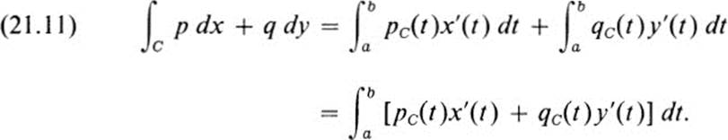
We next note that it is often convenient to combine a pair of line integrals of the form (21.3) and (21.4). Thus, given a curve C and a pair of continuous functions p(x, y), q(x, y) on C, we define ∫c p dx + q dy by
![]()
The left-hand side of Eq. (21.10) is a frequently used notation for the sum of the two integrals on the right.
We note first that the combined form ∫c p dx + q dy includes both of the line integrals (21.3) and (21.4) as special cases, by choosing either p = f and q = 0 or p = 0 and q = f. There is a more important reason for considering the sum (21.10) rather than each integral separately. Recalling the definition in Eqs. (21.3) and (21.4), we find
The integrand on the right-hand side has the form of a scalar product. From our discussion in Sect. 3, we recognize the vector
![]()
where s is the parameter of arc length along C, and T(t) is the unit tangent to C at the point x(t), y(t). If we introduce at each point of the curve the vector
![]()
then Eq. (21.11) takes the form
![]()
where L is the length of the curve C. The integrand v · T is equal to the component of the vector v in the direction of the unit vector T, or the tangential component of v; it is frequently denoted by υT. Equation (21.12) then takes the form

In order to guarantee the existence of the unit tangent T it is necessary to assume that C is a regular curve. We may then describe Eq. (21.13) as follows (Fig. 21.3). Let C be a regular curve of length L, and let s denote the parameter of arc length along C. To each point of C is assigned a vector v whose x and y components, p and q, vary continuously along C. Then the tangential component υT is a continuous function of s, and the ordinary integral of this function from 0 to L is equal to the line integral (21.10).
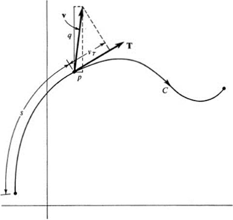
FIGURE 21.3 Geometric interpretation of ∫c p dx + q dy = ![]() ds
ds
Remark In analogy with Eqs. (21.3)and (21.4), we define ∫c f ds, the integral of f with respect to arc length, by
By the chain rule, we have
where the integrand on the right is simply the function f referred to the parameter of arc length s. In this notation Eq. (21.13) takes the form

Example 21.4
Consider the case where the components of v are constant. Let us set v = ![]() c,d
c,d![]() , where |v| = 1. Then for the curve C defined by (21.1), we have
, where |v| = 1. Then for the curve C defined by (21.1), we have
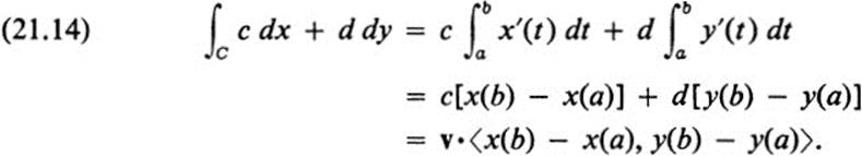
The right-hand side of Eq. (21.13) may be described in this case as the integral of the component of the unit tangent T in the direction of the fixed unit vector v, and the result yields, by Eq. (21.14), the projection in the direction of vof the displacement vector from the initial point to the endpoint of C.
An interesting feature of Example 21.4 is that if we consider the constant vector field v(x, y) = ![]() c, d
c, d![]() ; defined in the whole plane, and compute the line integral (21.14) for different choices of the curve C, then the resulting value depends only on the initial point and the endpoint of C, and is completely independent of the path taken by C in between. We shall encounter independence of path in a more general setting in the next section.
; defined in the whole plane, and compute the line integral (21.14) for different choices of the curve C, then the resulting value depends only on the initial point and the endpoint of C, and is completely independent of the path taken by C in between. We shall encounter independence of path in a more general setting in the next section.
We conclude the present section with a brief discussion of the interpretation of the line integral in the case where the vector v = ![]() p, q
p, q![]() has one of the physical interpretations discussed at the end of Sect. 19.
has one of the physical interpretations discussed at the end of Sect. 19.
First, consider the case where v represents a force, and C is the trajectory of a particle that is subjected at each point to the force v. Then υT represents the component of the force in the direction of motion, and the integral ![]() dsis defined in physics to be the work done by the force in moving the particle along the path C. By Eq. (21.13), this physical quantity is represented by a line integral in terms of the components p and q of the force at each point. From Eq. (21.14) we see that in the special case where the force is constant and the partial moves along a straight line in the direction of the force, the work done is equal to the magnitude of the force times the distance traversed. It follows from the same equation that if the force is constant, but the path is not straight, the work done depends not on the distance traversed, but on the displacement between beginning and endpoint (which is not at all evident on physical grounds).
dsis defined in physics to be the work done by the force in moving the particle along the path C. By Eq. (21.13), this physical quantity is represented by a line integral in terms of the components p and q of the force at each point. From Eq. (21.14) we see that in the special case where the force is constant and the partial moves along a straight line in the direction of the force, the work done is equal to the magnitude of the force times the distance traversed. It follows from the same equation that if the force is constant, but the path is not straight, the work done depends not on the distance traversed, but on the displacement between beginning and endpoint (which is not at all evident on physical grounds).
The second physical interpretation is that of a fluid flow, where v is the velocity vector of the flow at each point. Then υT represents the component of the flow velocity in the direction of the curve C, and ![]() may be described as the “total rate of flow along C.”
may be described as the “total rate of flow along C.”
Exercises
21.1 Let f(x, y) = x2 − y2. Compute the line integrals ∫c f dx for the following curves.
a. ![]()
b. ![]()
c. ![]()
d. ![]()
21.2 Verify Lemma 21.1 for the case f(x, y) = xy, where
![]()
and
![]()
so that
![]()
21.3 Verify Lemma 21.2 for the case f(x ,y) = 1 /x, where
![]()
21.4 Evaluate ∫c y dx — x dy for each of the following curves.
a. ![]()
b. ![]()
c. ![]()
d. C is the straight-line segment from (0, 0) to (1, 1).
e. C is the straight-line segment from (1, 1) to (0, 0).
21.5 Evaluate ∫c y dx + x dy for each of the curves of Ex. 21.4.
21.6 Evaluate
![]()
where
a. C is the upper arc of the circle x2 + y2 = 2 going from (1, 1) to
(−1,1).
b. C is the straight-line segment from (1, 1) to (−1, 1).
c. C is the lower arc of the circle x2 + y2 = 2 going from (1,1) to (−1, 1)
21.7 For each of the following vector fields v(x, y), evaluate ∫ c υT ds, where C is the ellipse,
![]()
a. v = ![]() x, y
x, y ![]()
b. v = ![]() x, y
x, y![]()
c. v = ![]() −y,x
−y,x![]()
d. v = ![]() − x, y
− x, y ![]()
e. v = ![]() y, 0
y, 0 ![]()
f. v = ![]() 0, y
0, y ![]()
g. v = ![]() c, d
c, d ![]() , c and d are constant
, c and d are constant
21.8 Explain how the answer to Ex. 21.7g could be predicted by Eq. (21.14).
21.9 Evaluate ![]() ds, where v is the vector field of Ex. 21.7c, and
ds, where v is the vector field of Ex. 21.7c, and ![]() is the ellipse
is the ellipse
![]()
Compare your answer with the answer to Ex. 21.7c and explain how it could have been predicted.
21.10 Show that if a curve C lies on a vertical line, then for any function f(x, y), ∫c f dx = 0. If C lies on a horizontal line, then ∫c f dy = 0 for any f.
21.11 Let C be defined by x = φ(t) ψ(t), y = ψ(t), a ≤ t ≤ b. Choose values t0, t1, …, tn such that
![]()
Let Ck be the curve defined by x = φ(t), y = ψ(t), tk-1 ≤ t ≤ tk, where k = 1,2, …, n.
a. Draw a sketch indicating the curves C1 …, Cn and their relation to C.
b. Show that for any function f(x, y),
![]()
![]()
![]()
*21.12Let C be a curve defined by x = φ(t), y = ψ(t), a ≤ t ≤ b.
a. if φ’(t) > 0 for a ≤ t ≤ b, show that the equation x = φ(t), a ≤ t ≤ b can be inverted in the form t = h(x), α ≤ x ≤ β.
b. In the notation of part a, if g(x) = ψ (h(x)) show that
![]()
c. Define F(x) by F(x) = f(x, g(x)), α ≤ x ≤ β. Note that the equation y = g(x) is simply the nonparametric form of the curve C. Draw a sketch illustrating the function F(x) as follows. Draw the curve C in the form y = g(x). For each value of x, α ≤ x ≤ β, erect a line perpendicular to the x axis and find the point (x,y) where this line intersects the curve C. Then F(x) is the value of f at this point (x, y). By part b, the ordinary integral of the function F(x) with respect to x is equal to the line integral ∫c f dx. (This could also be described in terms of Lemma 21.1 as making a change of parameter such that ![]() is the curve x = τ, y = g(τ), α ≤ τ ≤ β.)
is the curve x = τ, y = g(τ), α ≤ τ ≤ β.)
d. If φ'(t) < 0 for a ≤ t ≤ b, then setting t = a + b(1 − τ), 0 ≤ τ ≤ 1, we obtain a new curve ![]() defined by x = φ(τ) = φ(t(τ)), y = ψ(τ) = φ(t(τ)), which consists of the curve C described in the opposite direction. Using parts a and b and Lemmas 21.1 and 21.2, show that
defined by x = φ(τ) = φ(t(τ)), y = ψ(τ) = φ(t(τ)), which consists of the curve C described in the opposite direction. Using parts a and b and Lemmas 21.1 and 21.2, show that
![]()
where y = g(x), α ≤ x ≤ β is the nonparametric form of the curve ![]() .
.
e. Combining parts a – d we may form the following picture of a line integral ∫c f dx. If C1 is a part of the curve C along which x is an increasing function of t, then ∫c1 f dx is the ordinary integral with respect to x of fconsidered as a function of its x coordinate alone along the curve C1. If C2 is a part of the curve along which x is a decreasing function of t, then let ![]() be the curve C2 described in the opposite direction, ∫c2 f dx = —
be the curve C2 described in the opposite direction, ∫c2 f dx = — ![]() f dx and the latter integral may be described as above. Finally, if C3 is a part of the curve on which x is constant, then ∫C3 f dx = 0. Describe in analogous fashion ∫c f dy.
f dx and the latter integral may be described as above. Finally, if C3 is a part of the curve on which x is constant, then ∫C3 f dx = 0. Describe in analogous fashion ∫c f dy.
21.13 Evaluate ∫c f ds for the following functions f(x, y) and curves C.
a. f(x, y) = y, C is the straight-line segment from (0, 1) to (1, 0).
b. f(x, y) = x2 + y2, C is the circle x = 2 cos t, y = 2 sin t, 0 ≤ t ≤ 2π.
c. f(x, y) = (1 − x2 − y2)1/2, C the same as in part a.
d. f(x, y) = y, C the straight-line segment from (1,0) to (0, 1).
e. f(x,y) = xy, C is the part of the ellipse x2/a2 + y2/b2 = 1, lying in the first quadrant.
21.14 Prove that ∫c f ds does not depend on the orientation of the curve C; that is, given a curve
![]()
let ![]() be the curve obtained from C by setting
be the curve obtained from C by setting
![]()
Show that
![]()
(Hint: follow the proof of Lemma 21.2, but note carefully the form of the chain rule for ds/dt; the equation
![]()
is not always true. What is the correct form of this equation?)
RemarkThe ordinary integral of a function of a single variable, ![]() F(x) dx, has a well-known geometric interpretation in terms of area. The line integral ∫c f ds may also be pictured in terms of areas, but in this case the interpretation is in terms of areas of curved surfaces. Since the surfaces involved are of special kinds, rather than general curved surfaces, it is possible to obtain an intuitive picture without having studied the general theory. In Exs. 21.5-21.7 we discuss some of the relationships between the line integral and the area of certain surfaces. The facts stated concerning the area of these surfaces follow easily from the general theory of surface area. (See, for example, the discussion of surface area in [11], Chapter IV, section 6.)
F(x) dx, has a well-known geometric interpretation in terms of area. The line integral ∫c f ds may also be pictured in terms of areas, but in this case the interpretation is in terms of areas of curved surfaces. Since the surfaces involved are of special kinds, rather than general curved surfaces, it is possible to obtain an intuitive picture without having studied the general theory. In Exs. 21.5-21.7 we discuss some of the relationships between the line integral and the area of certain surfaces. The facts stated concerning the area of these surfaces follow easily from the general theory of surface area. (See, for example, the discussion of surface area in [11], Chapter IV, section 6.)
21.15 Let C be a curve x(t), y(t), a ≤ t ≤ b, and let f(x, y) be a function that is defined and continuous along C. Assume further that f(x, y) ≥ 0 on C. Using rectangular coordinates x,y,z in three-dimensional space, consider the curve C to lie in the x, y plane, and erect above each point (x, y) of C, the vertical line segment of height f(x, y). As the point (x, y) traces out the curve C, from (.x(a), y(a)) to (x(b), y(b)), these vertical line segments sweep out a “cylindrical surface” S. The area of this surface S is equal to ∫c f ds.
a. Draw a sketch illustrating the curve C and the surface S just described.
b. If the function f(x, y) is defined in a domain D in which the curve C lies, the surface S may be described as “the surface lying above the x, y plane and below the space curve defined as the intersection of the surface z = f(x, y) with the cylindrical surface generated by all vertical lines through C.” Illustrate this with a sketch.
c. Explain Ex. 21.14 (at least for positive functions f ) in terms of this geometric interpretation of the line integral.
*d. Using this interpretation, show that the answers to Ex. 21.13a, b, and c consist of the areas of a triangle, cylinder, and semicircle, respectively. Use elementary geometry to compute these areas, and verify the results obtained previously.
21.16 Using the geometric interpretation of the line integral given in Ex. 21.15, find the area of the cylindrical surfaces S described as follows, and illustrate each surface with a sketch.
a. S lies over the circle x2 + y2 = 1 and under the surface z = 1 + x2.
b. S lies over the circular arc x = a cos t, y = a sin t − ![]() ≤ t ≤
≤ t ≤ ![]() , and under the surface z = x2 − y2.
, and under the surface z = x2 − y2.
c. S lies over the elliptic arc y = 2(1 −x2)1/2, 0 ≤ x ≤ 1, and under the surface z = xy.
*d. S is the part of a circular cylinder of radius a cut out by another cylinder of equal radius, the axes of the two cylinders intersecting at right angles.
*e. Consider a vertical cylinder of radius ![]() whose axis intersects the y axis at the point (0,
whose axis intersects the y axis at the point (0, ![]() ). S is that part of the cylinder which lies in the first octant and is cut out by a sphere of radius 1 with center at the origin.
). S is that part of the cylinder which lies in the first octant and is cut out by a sphere of radius 1 with center at the origin.
21.17 Let C be a curve of the form y = g(x), a ≤ x ≤ b where g(x) ≥ 0 for a ≤ x ≤ b. Let S be the surface obtained by revolving the curve C about the x axis. Then S is a surface of revolution, and its area A is given by the formula
![]()
Use this formula to compute the area of the following surfaces, and sketch each surface.
a. A cone, where C: x = ht, y = rt, 0 ≤ t ≤ 1.
b. A frustrum of a cone, C: y = ((r2 - r1)/h)x + r1 0 ≤ x ≤h show that the area of the cone of part a, and that of a circular cylinder may both be obtained as special cases.
c. A paraboloid of revolution; C: y = ![]() , 0 ≤ x ≤ 2.
, 0 ≤ x ≤ 2.
d. A zone of a sphere; C: y = ![]() h1, ≤ x ≤ h2.
h1, ≤ x ≤ h2.
(Note the curious fact that the area depends only on the width of the zone.)
e. A catenoid; C: y = cosh x (a catenary), − h ≤ x ≤ h.
*f. A pseudosphere ; C is defined for x > 0 to be a curve y = g(x),where at each point
and g(0) = a (the tractrix). It has the properties g(x) > 0 for x > 0 and limx→∞g(x) = 0. If this curve is reflected in the y axis by setting g( − x) = g(x), and the entire curve thus obtained is revolved about the x axis, the resulting surface is called the pseudosphere of pseudoradius a. Show that for any x1, x2 such that 0 < x1 < x2, the zone of the pseudosphere satisfying x1 ≤ x ≤ x2 has surface area 2πn[g(X1) —g(x2)].
g. By taking the limit as x1 tends to zero and x2 tends to infinity in part f, find the area of the entire pseudosphere, and compare with the area of the entire sphere obtained by setting h1 = − a, h2 = a in part d.
21.18 A physical interpretation of the line integral ∫c f ds is the following. Picture a wire of variable density bent into the shape of the curve C. If the density at each point (in mass per unit length) is equal to f then the total mass of the wire is equal to ∫c f ds. Compute the total mass in each of the following cases.
a. f(x, y) = ![]() C: y = x2, 0 ≤ x ≤ 1
C: y = x2, 0 ≤ x ≤ 1
b. f(x, y) = |x| + |y| C: x = cos t, y = sin t, 0 ≤ t ≤ π
c. f(x, y) = ![]() C:x = et cos t, y = et sin t, −
C:x = et cos t, y = et sin t, −![]() ≤ t ≤
≤ t ≤ ![]()
d.f(x, y) = ![]() C:x = t − sin t, y = 1 — cos t, 0 ≤ t ≤ 2π
C:x = t − sin t, y = 1 — cos t, 0 ≤ t ≤ 2π
21.19 In the notation of Ex. 21.18, where f(x, y) represents the density in mass per unit length, the following quantities have physical importance. (For the corresponding quantities in the case of plane figures, see Ex. 24.12.,
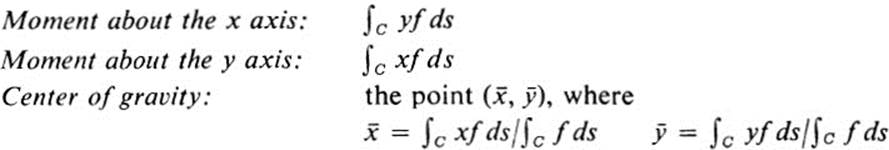
For each part of Ex. 21.18, compute both moments, and use them to find the center of gravity.
21.20 If in Ex. 21.19, the density f is constant, then this constant cancels out in the definition of ![]() and
and ![]() , and hence the center of gravit
, and hence the center of gravit![]() depends only on the curve C; it is called the centroid of the curve C, and is given by
depends only on the curve C; it is called the centroid of the curve C, and is given by ![]() , with
, with
![]()
where L is the length of C. Find the centroid of each of the following curves C.
a. The circular arc: x = cos t, y = sin t, 0 ≤ t ≤ α.
b. The straight-line segment from (x1, y1) to (x2, x2).
*c. The first arch of the cycloid: x = t — sin t, y = 1 — cos t, 0 ≤ t ≤ 2π.
d. The first quadrant of the hypocycloid or astroid: x = cos3t, y = sin3t, 0 ≤ t ≤ ![]() .
.
21.21 Let S be a surface of revolution formed by revolving a plane curve C about a fixed line that does not cross the curve. Let R be the distance of the centroid of C from the fixed line, and let L be the length of the curve C. The Theorem of Pappus states that the area A of the surface S is given by the formula
![]()
a. Prove the theorem of Pappus. (Note that it may be assumed that the curve C lies in the upper half-plane and that the fixed line coincides with the x axis.)
b. Verify the theorem of Pappus for the case of a frustrum of a cone, by comparing the answers to Exs. 21.17b and 21.20b.
c. Use the theorem of Pappus and the centroid of the circle,
![]()
to find the surface area of the torus obtained by revolving the circle C about the x axis.
d. Use the theorem of Pappus and the known area of a sphere (Ex. 21.17d) to find the centroid of a semicircle, x2 + y2 = a2, y ≥ 0.
21.22 In each of the following cases interpret the vector field v =
a. v = ![]() x − y, x + y
x − y, x + y ![]() ; C:x = cos t, y = sin t, 0 ≤t ≤π
; C:x = cos t, y = sin t, 0 ≤t ≤π
b. v = ![]() x2 + y2, x2 −y2
x2 + y2, x2 −y2 ![]() ; C:x = cos t, y = sin t, 0 ≤t ≤π
; C:x = cos t, y = sin t, 0 ≤t ≤π
c. v = ![]() 6xy2,5xy −2
6xy2,5xy −2![]() ; C:y = x2, 0 ≤ x ≤ 1
; C:y = x2, 0 ≤ x ≤ 1
d. v = ![]() 1, x
1, x![]() ; C:y = log x, 1 ≤x≤2
; C:y = log x, 1 ≤x≤2
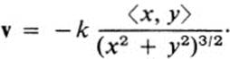
21.23 According to the “inverse square law,” the force exerted is inversely proportional to the square of the distance from the body exerting the force. If that body is placed at the origin, the field takes the form
a. Find the work done by this force in moving a particle along a straight- line segment from the point (r2 cos α, r2 sin α) to (r1 cos α, r1 sin α), where α is fixed and r1 < r2.
b. Find the work done in moving a particle along a horizontal line segment from (r2 cos α, r2 sin α) to (r1 cos α, r2 sin α).
c. Find the work done in moving a particle along a vertical line segment from (r1 cos α, r2 sin α) to (r1 cos α, r1 sin α).
d. Show that the total work done in parts b and c is the same as the work done in part a.
e. Let C be a path consisting of an arbitrary succession of horizontal and vertical line segments, starting at a point whose distance from the origin is R2 and ending at a point whose distance from the origin is R1. Show that the total work done in moving a particle along the path C is equal to k(1/R1 — 1/R2). (Hint: show that this is true for each of the line segments making up the path, and deduce that it must be true for the whole path.)
*21.24 The definition we have given of line integrals is best suited for the actual computation of line integrals, but it has two theoretical disadvantages. First, it was expressed in terms of the parameter t, and we had to show later that the value of the line integral was actually independent of the choice of parameter. Second, the definition can only be applied to differentiable curves. There is an alternative definition, which avoids both of these difficulties. Given a curve C with a fixed orientation and a function f(x, y) continuous on C, choose an arbitrary sequence of points (xn, yn) along C (ordered according to the given orientation). Let (ξn,ηn) be an arbitrary point on C between (xn-1, y n-1) and (xn, yn). Use the notation
![]()
Form the sums
![]()
If these sums tend to a limit as the maximum of Δsn tends to zero, this limit being independent of the subdivision and of the choice of intermediate points (ξn,ηn), then the limits are defined to be
![]()
respectively.
a. Draw a sketch indicating the quantities Δxn, Δyn, Δsn and the point(ξn,ηn)
b. For C a differentiable curve, so that x and y are differentiable functions of a parameter t, write down the above sums in terms of t by applying the mean value theorem for functions of one variable to the terms Δxn and Δyn. Show that it is reasonable to expect these sums to tend in the limit to the expressions we used to define the corresponding line integrals.
21.25 The line integrals
![]()
which we have defined in this section, are special cases of a more general situation. Suppose that f(x,y) and g(x, y) are defined along C. We wish to define ∫c f dg. This may be done in the manner described in Ex. 21.24, or else, in case g'c(t)exists and is continuous, we may follow the procedure used in Eqs. (21.3) and (21.4) , and use as our definition
![]()
In particular, if C is a differentiable curve lying in a domain D, if g(x, y) ∈![]() in D, and if f(x, y) is continuous along C, then the integral on the right exists, and we use it to define ∫c f dg. An important case is that in which the curve C does not pass through the origin, and we choose for g(x, y) one of the functions
in D, and if f(x, y) is continuous along C, then the integral on the right exists, and we use it to define ∫c f dg. An important case is that in which the curve C does not pass through the origin, and we choose for g(x, y) one of the functions
![]()
Note that any two branches of θ(x, y) differ by a constant, and therefore the expression
![]()
is well-defined for each t. Thus the line integrals
![]()
are uniquely defined, independently of how θ itself is chosen along any part of the curve C.
In case the function f(x, y) ≡ 1, we use the notation
![]()
a. Suppose that C does not pass through the origin. Show that
![]()
b. Under the same hypotheses as part a, show that
![]()
c. Show that
![]()