Two-Dimensional Calculus (2011)
Chapter 4. Integration
22. Potential functions; independence of path
In the previous section we computed line integrals by first expressing them as ordinary (definite) integrals, and then evaluating these integrals in the usual fashion by finding indefinite integrals; that is, by using the fundamental theorem of calculus. In the present section we prove a theorem that may be considered to be a generalization of the fundamental theorem of calculus to functions of two variables. We replace definite integrals by line integrals, and indefinite integrals or antiderivatives by potential functions. One consequence is a rapid method of evaluating many line integrals.
We begin by stating the two standard forms of the fundamental theorem of calculus.2
Let g(x) be continuous on an interval a ≤ x ≤ b. Then


We can summarize these two statements by saying “differentiation and integration are inverse processes.” We shall show that in a certain sense “forming gradients and line integrals are inverse processes.” To be made precise, this rough statement must be separated into several parts. We start with a result generalizing Eq. (22.2).
Lemma 22.1 Let f(x, y ) ∈ ![]() in a domain D. Consider the gradient vector field
in a domain D. Consider the gradient vector field
![]()
in D. Let (x2, y2)(x2, y2) be any two points in D, and consider a differentiable curve
![]()
lying in D, such that
![]()
Then

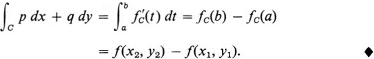
PROOF. By definition of the line integral,

But by (22.3) and Th. 7.1, we have at each point of the curve C
![]()
Whence, by (22.2)and(22.5)
Remark Recalling that a function f satisfying (22.3) in a domain is called a potential function for the vector field ![]() p,q
p,q![]() , we may state the content of Lemma 22.1 as follows: if a vector field
, we may state the content of Lemma 22.1 as follows: if a vector field ![]() p, q
p, q![]() has a potential function f in a domain D, then for any curve C lying in D, the value of the line integral ∫c p dx + q dy is obtained by simply forming the difference between the values of f at the endpoint and at the beginning point of C.
has a potential function f in a domain D, then for any curve C lying in D, the value of the line integral ∫c p dx + q dy is obtained by simply forming the difference between the values of f at the endpoint and at the beginning point of C.
Example 22.1
Consider Eq. (21.14). There the vector field v was constant, v = ![]() c, d
c, d![]() . We may set v = Δf, where f = cx + dy. Then by Eq. (22.6),
. We may set v = Δf, where f = cx + dy. Then by Eq. (22.6),
![]()
which, by virtue of (22.5), is the same as the result obtained previously.
Example 22.2
Evaluate ∫ c y dx + x dy, where
![]()
Method 1. Using the definition of the line integral, since x'(t) = − sin t, y'(t) = cos t,

Method 2. Using Lemma 22.1, with p = y, q = x, clearly the function f(x, y) = xy satisfies (22.3). Since the curve C starts at (1,0) and ends at (0, 1), we have by (22.6)
![]()
For various applications it is desirable to enlarge the class of curves C over which we form line integrals, and to observe that Lemma 22.1 continues to hold for this wider class of curves.
Definition 22.1 A piecewise smooth curve is a curve C:x(t ), y(t), a ≤ t ≤ b, where x(t), y(t) are continuous for a ≤ t ≤ b, and where there exist a finite number of values t1 < t2 < ··· . < tn between a and b such that x(t), y(t) define a regular curve on each of the intervals
![]()
Remark When referring to a differentiable function on a closed interval, it is understood that only the right- or left-hand derivative is defined at the endpoints. Thus, for a piecewise smooth curve, the functions x(t) and y(t)in general have distinct right- and left-hand derivatives at the points tk. Geometrically speaking, a piecewise smooth curve is allowed to have a finite number of corners.
Definition 22.2 If C is a piecewise smooth curve as defined above, and if p(x, y), q(x, y) are continuous along C, then ∫c p dx + q dy is defined by

where
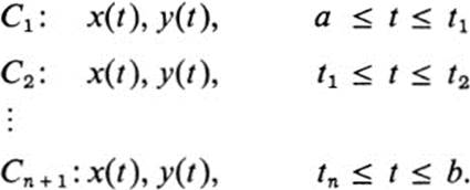
Lemma 22.2lemma 22.1 remains true if we allow C to be any piecewise smooth curve lying in D
PROOF. Applying Lemma 22.1 to each of the curves C1,…, Cn + 1, in the notation of Def. 22.2 and adding, we find
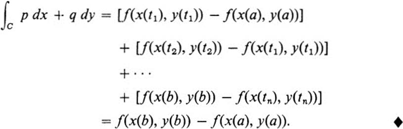
This is the desired generalization of the fundamental theorem of calculus in its second form. Thus, we may state Eq. (22.2) in the following form: the integral of the derivative of a function over an interval yields the difference in values of the function at the endpoints of the interval. The corresponding statement for a function of two variables takes the form: the line integral of the gradient of a function over a curve yields the difference in values of the function at the endpoints of the curve. Let us recall also that the proof of the second statement consists essentially in reducing it to the first one by our familiar device of forming the function fc(t) of a single variable out of a function f(x, y) of two variables restricted to the curve C.
We turn next to the problem of generalizing statement (22.1). In essence, this statement may be paraphrased as follows: the definite integral of a function over an interval with fixed initial point and variable endpoint yields a function of the variable endpoint whose derivative is the original function. In two variables, the corresponding problem would be to find a function having given partial derivatives, and if possible, to do so by representing this function as an integral with variable endpoint. We shall divide this problem into two parts—one for the x derivative and one for the y derivative.
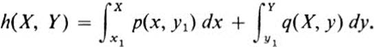
Lemma 22.3 Let p(x,y ), q(x, y) be arbitrary continuous functions in a disk D: (x − x1)2 + (y − y12) < r2. For each point (X, Y) in D, define g(X, Y) as follows: let C be the piecewise smooth curve consisting of the vertical line segment from (x1, y1) to (x1, y) followed by the horizontal line segment from (x1, y) to (x, y) (see Fig. 22.1). Set

Then at each point of D,
![]()
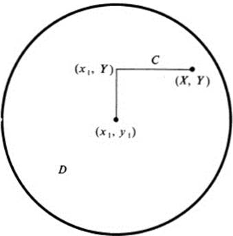
FIGURE 22.1 Notation for Lemma 22.3
PROOF. If we denote the vertical line segment by Cl, and the horizontal one by C2, then along Cl x ≡ xl and dx/dt ≡ 0, whatever the choice of the parameter t. Similarly, along C2, dy/dt ≡ 0. If we then make a change of parameter so that along C1 we use simply y as the parameter, and along C2 we use x, we have
To form ∂g/∂X we hold Y fixed and take the ordinary derivative with respect to X. But with Y fixed, the first term on the right is a constant, whereas the second term on the right becomes the integral of a function of the single variable x, over an interval with fixed initial point and variable endpoint. Application of (22.1) therefore gives
![]()
which is the desired result, Eq.(22.8). ![]()
Remark The fact that D was a disk, rather than an arbitrary domain, was needed to guarantee that the curve C lay entirely in D for any choice of (X, Y). It may appear that by choosing C in a different manner the proof could be made to work in any domain D. However, given a continuous function p(x, y) in an arbitrary domain D, there may not exist a continuous function g(x, y) in D satisfying (22.8). An analogous statement holds for Eq. (22.10). For further details, see Ex. 22.18.
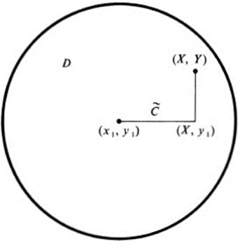
FIGURE 22.2 Notation for Lemma 22.4
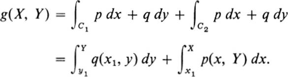
Lemma 22.4 Using the same notation as in Lemma 22.3, let ![]() be the curve consisting of the horizontal segment from (x1, y1) to (x, y1) followed by the vertical segment from (X, y1) to (X, Y) (Fig. 22.2). Set
be the curve consisting of the horizontal segment from (x1, y1) to (x, y1) followed by the vertical segment from (X, y1) to (X, Y) (Fig. 22.2). Set

then
![]()
PROOF.As in Lemma 22.3, we find
Fixing X and letting Y vary, the first term becomes constant and we may apply (22.1) to the second term, yielding (22.10). ![]()
Combining the statements of these two lemmas, we may summarize the situation as follows: given an arbitrary continuous function in a neighborhood of a point (x1, y1) we can find a function g(X, Y) in this neighborhood having the given function as its X derivative, and another function h(X, Y ) having the given function as its Y derivative. Furthermore, each of the functions g(X, Y), h(X, Y) is represented as a line integral from the fixed point (x1,y1) to the variable point (X, Y).
The next question that arises is whether we can construct a single function, having prescribed both partial derivatives. We know already from Lemma 19.1 that the answer is, in general, “no.” There does not exist, for example, a function f(x, y) satisfying simultaneously
![]()
since it would follow that on the one hand fxy = 2y and on the other hand fxy = 2x. In general, if p(x, y), q(x, y) ∈ ![]() , then it is impossible to have simultaneously
, then it is impossible to have simultaneously
![]()
unless py = qx.
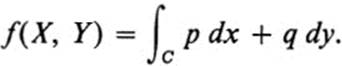
It is important to observe that if, for given p and q, there does exist a function f(x, y) satisfying (22.11), then this function may be represented by a line integral. Namely, if p(x, y), q(x, y) are continuous in a domain D, and if there exists a function f(x, y) in D satisfying (22.11), then for any fixed point (x1, y1) in D, and for a variable point (X, Y), if we let C be a curve in D starting at (x1 y1) and ending at (X, Y), Lemma 22.1 shows that
![]()
One consequence of Lemma 22.1 is that for vector fields possessing a potential function, the value of the line integral over a curve C depends only on the beginning and endpoint of C. This property of a vector field has a special designation.
Definition 22.3 Let p(x, y), q(x, y) be continuous in a domain D. The line integral ∫c p dx + q dy is called independent of path if for any two piecewise smooth curves C1, C2, lying in D and having the same beginning and endpoints,

Combining Lemmas 22.2, 22.3, and 22.4, we arrive at the following fundamental result.
Theorem 22.1 Let p(x, y), q(x, y) be continuous functions in a domain D. Then the following are equivalent:
1. there exists a function f(x, y) in D satisfying (22.11);
2. ∫c p dx + q dy is independent of path.
PROOF. It follows immediately from Lemma 22.2 that the first statement implies the second. To prove the converse, let (x0, y0) be any fixed point of D. For an arbitrary point (X, Y) in D, let C be a piecewise smooth curve starting at (x0, y0) and ending at (X, Y). By assumption, the value of ∫c p dx + q dy does not depend on the choice of C, but only on the endpoint (X, Y). We may therefore write
Consider next an arbitrary point (xl, yl) in D and a neighborhood N of (x1,y1) such that N lies in D. For any point (X, Y) in N, we may choose the curve C to consist of a fixed curve C1 from (x0, y0) to (x1 y1) followed by a vertical line segment C2 followed by a horizontal segment C3. Then
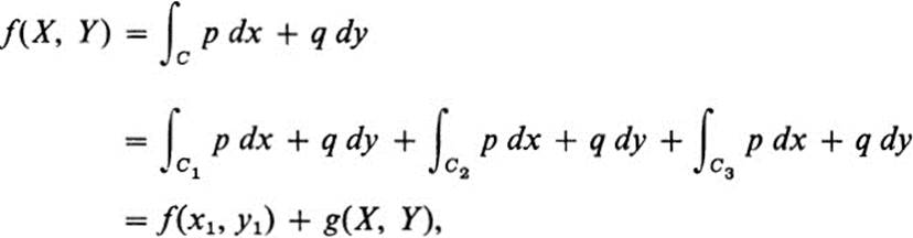
where g(X, Y) is the function defined in Lemma 22.3. It follows from Lemma 22.3 that fx(X, Y) = gx(X, Y) = p(X, Y) at all points of N, and in particular, at (x1, y1). Similarly, we may choose C to consist of C1 followed by a horizontal segment ![]() followed by a vertical segment
followed by a vertical segment ![]() Then, in the notation of Lemma 22.4,
Then, in the notation of Lemma 22.4,
![]()
throughout N. Since (x1 y1) was an arbitrary point of D, it follows that (22.11) is satisfied throughout D, and the theorem is proved. ![]()
It is often convenient to treat the notion of independence of path in a slightly modified form.
Definition 22.4 A curve C:x(t), y(t) a ≤ t ≤ b, is called closed if (x(b), y(b)) = (x(a), y(a)) ; that is, if its endpoint is the same as its beginning point.
Lemma 22.5 Let p(x, y), q(x, y) be continuous in a domain D. Then the following are equivalent:
1. ∫c p dx + q dy is independent of path ;
2. ∫c p dx + q dy = 0 for every piecewise smooth closed curve C lying in D.
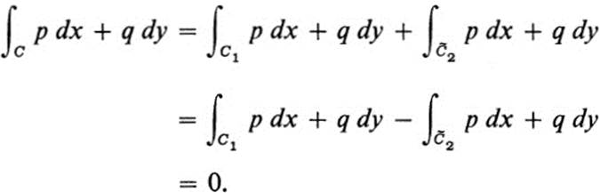
PROOF. Assume that the first condition holds, and let C:x(t), y(t), a ≤ t ≤ b, be any closed curve in D, where x(a) = x(b) = x0, y (a) = y(b) = y0. Let C1 and C2 be the parts of C corresponding to the parameter values a ≤ t ≤ (a + b)/2 and (a + b)/2 ≤ t ≤ b, respectively. Let ![]() be the curve C2 traversed in the opposite direction. Then C1 and
be the curve C2 traversed in the opposite direction. Then C1 and ![]() have the same beginning and endpoints, so that
have the same beginning and endpoints, so that
Conversely, suppose that the second condition holds. Let C1 and C2 be any two curves in D starting at the same point (xl ,y1), and ending at the same point (x2, y2). Let ![]() consist of the curve C2 traversed in the opposite direction. Then the curve C consisting of C1 followed by
consist of the curve C2 traversed in the opposite direction. Then the curve C consisting of C1 followed by ![]() is a closed curve starting and ending at (x1, y1), By virtue of Lemma 21.2 we have
is a closed curve starting and ending at (x1, y1), By virtue of Lemma 21.2 we have
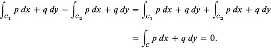
But this is just the condition (22.12) for independence of path, and the lemma is proved. ![]()
Example 22.3
Consider the vector field

defined in the domain D consisting of the whole plane with the origin deleted. Consider the curve
![]()
Then C is a closed curve in D, starting and ending at (1, 0). On C we have
![]()
and therefore

Thus the second condition of Lemma 22.5 fails to hold for the vector field (22.13), and consequently the first condition also fails. It follows from Th. 22.1 that there cannot exist a potential function for this vector field. On the other hand, by direct verification, the condition py = qx does hold throughout D. We thus have an example that shows that the converse of Lemma 19.1 is not true.
If we now combine Lemma 22.5 with Th. 22.1 and Lemma 19.1, we arrive at the following result.
Theorem 22.2Let p(x, y),q(x, y) ∈ ![]() in a domain D,then
in a domain D,then
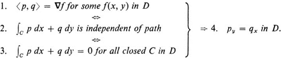
Thus the first three conditions are equivalent, and each of them implies the fourth. Condition 4 does not imply the first three, as the example just given shows.
It is illuminating to examine the content of this theorem in the light of various physical interpretations of the vector field v = ![]() p, q
p, q ![]() .
.
Consider, first, the case where v represents a force field. Then, as we have indicated in Sect. 21, the line integral ∫ c p dx + q dy represents work. The line integral’s independence of path is interpreted to mean physically that the work done in moving a particle from one point to another is independent of the choice of path. In this case we can assign a “potential energy” to each point of the field, such that the difference in potential energy at any two points represents the work done by the field in moving a unit particle from the point of higher potential to one of lower potential, or equivalently, the work that has to be done against the field to move the particle from the point of lower potential to that of higher potential. Thus, lifting a weight through a certain height against the force of gravity is often interpreted as increasing the weight’s potential energy, which can be converted back into work by letting the weight drop. In the proof of Th. 22.1, we have seen that potential energy defined in this way is precisely a potential function for the vector force field, that is to say, a function f(x, y) satisfying (22.3). It is from this application that the terminology derives. Condition 3 of Th. 22.2 is also easily interpreted in these terms. It states that it is impossible to increase the potential energy by following some trajectory and returning to the starting point. This is one form of the so-called “law of conservation of energy,” and it is in this connection that the term “conservative vector field” arose, indicating a vector field satisfying the equivalent conditions 1, 2, 3 of Th. 22.2.
We turn next to the interpretation of the vector field v as the velocity field of a fluid flow. In that case we noted that the line integral ∫ c p dx + q dy may be interpreted as the total rate of flow along the curve C. If C is a closed curve, the line integral would represent the total rate of flow around the curve C. For this reason, a fluid flow satisfying condition 3 of Th. 22.2 (and hence the equivalent conditions 1 and 2) is called irrotational, and the same word is used to denote an arbitrary vector field having this property. Thus the designations “conservative” and “irrotational” indicate identical properties of a vector field, but arise from different applications.
In conclusion we note that the terms “conservative” and “irrotational” are frequently used for vector fields satisfying condition 4 of Th. 22.2. As we have seen, this condition is not strictly equivalent to the other three, and consequently there may be some confusion in using the same terms for different properties. The reason that distinct words were not chosen is that under certain restrictions all four properties in Th. 22.2 are equivalent. (See Th. 25.2and the discussion following it.) In order to show this it is necessary to introduce double integrals, which we shall define and study in the following sections.
Exercises
22.1 Evaluate each of the following line integrals by finding a potential function f(x, y) and applying Lemma 22.1.
a. ![]()
b. ![]()
c. ![]()
d. ![]()
e. ![]()
f. ![]()
22.2 Do Ex. 21.5, using Lemma 22.1.
22.3 Illustrate the definition of a piecewise smooth curve by a sketch.
22.4 Let C be the curve from (1, 1) to (3, 2) consisting of a horizontal segment C1 followed by a vertical segment C2.
a. Write C explicitly as a piecewise smooth curve.
b. Evaluate ∫ c x2y dx — 3x dy.
c. Evaluate ∫ c y2 dx + 2xy dy, first by a direct computation, and then by using Lemma 22.2.
22.5 Let C be the curve from (3, 2) to (1, 1) consisting of a horizontal line segment C1 followed by a vertical line segment C2. Answer parts a, b, and c of Ex. 22.4 for this curve.
22.6Let C be the rectangle consisting of the four successive line segments:
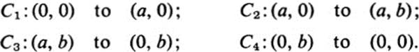
a.Write C explicitly as a piecewise curve
b.Evaluate ∫c x2 dx + y2 dy
c.Evaluate ∫ −c y dx + dy
22.7 Let ![]() p, q
p, q ![]() be a conservative vector field in a domain D. Then by the observation following Eq. (22.11), a potential function can be written down explicitly in the form of a line integral. If the domain D is of a simple type, such as a disk, or a rectangle, or the whole plane, then the path of integration can be chosen in a consistent simple way. For example, choosing the path consisting of a horizontal line segment followed by a vertical line segment, which joins (0, 0) to (X, Y), show that the function f defined by
be a conservative vector field in a domain D. Then by the observation following Eq. (22.11), a potential function can be written down explicitly in the form of a line integral. If the domain D is of a simple type, such as a disk, or a rectangle, or the whole plane, then the path of integration can be chosen in a consistent simple way. For example, choosing the path consisting of a horizontal line segment followed by a vertical line segment, which joins (0, 0) to (X, Y), show that the function f defined by
![]()
is a potential function.
22.8 Use the method of Ex. 22.7 to find potential functions for each of the following vector fields. (The domain D is the whole plane.)
a. ![]() 3x2y2 + 2xy3,3x2y2 + 2x3y
3x2y2 + 2xy3,3x2y2 + 2x3y ![]()
b.![]() 2x + 2xy − y, x2 − 3y2 − x
2x + 2xy − y, x2 − 3y2 − x ![]()
c.![]()
d. ![]() exy + xyexy, x2exy
exy + xyexy, x2exy![]()
22.9 Use the answers to Ex. 22.8 to evaluate the following line integrals.
a. ![]()
b. ∫c (2x + 2 xy − y) dx + (x2 − 3y2 − x) dy; C is the curve of Ex. 22.4
c. ![]()
d. ∫c (exy + xyexy) dx + x2exy dy; C: x = (y2 − 3)/2, −2 ≤ y ≤ 2.
22.10 Show that two vector fields may have the same direction at every point and one of the vector fields may be conservative, while the other one is not. (Hint: consider the effect on a vector field of multiplying through by a nonzero function.)
22.11 In each of the following cases we give a vector field ![]() p, q
p, q![]() and a function h. Show that the vector field
and a function h. Show that the vector field![]() p, q
p, q![]() is not conservative, but that the vector field
is not conservative, but that the vector field ![]() = h
= h![]() p, q
p, q ![]() =
= ![]() hp, hq
hp, hq![]() is. Find a potential function f for
is. Find a potential function f for ![]()
a. ![]() p,q
p,q![]() ; =
; = ![]() 3y, 6x − 3y
3y, 6x − 3y![]() ; h = y
; h = y
b. ![]() p,q
p,q![]() =
= ![]() y2,xy
y2,xy![]() ; h = 2x
; h = 2x
c. ![]() p, q
p, q![]() =
= ![]() y2,xy
y2,xy![]() ; h = x/(1 + x2y2)
; h = x/(1 + x2y2)
22.12 Let f(x, y) and g(x, y) be functionally dependent in a domain D. Show that the vector fields ∇f and ∇g have the same direction at every point where neither of them vanishes.
22.13 Let u(x, y) be a harmonic function in a domain D. A function υ(x, y) in D is called a conjugate harmonic function to u(x, y) if u and υ satisfy the Cauchy- Riemann equations ux = υy, uy = − υx. Given u(x, y) the problem of finding a conjugate harmonic function is equivalent to that of finding a potential function υ(x, y) for the vector field ![]() p, q
p, q![]() =
= ![]() − uy, ux
− uy, ux ![]() . Thus, a conjugate harmonic function can often be found by the method of Ex. 22.7. Carry this out for the following functions.
. Thus, a conjugate harmonic function can often be found by the method of Ex. 22.7. Carry this out for the following functions.
a. u = x − y
b. u = x2 − y2
c. u = sin x sinh y
d. u = cos x cosh y
e. u = ex cos y
f. u = x3y − xy3
22.14 Consider the vector field arising from a force that obeys the inverse square law
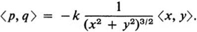
According to Ex. 21.23e, if (x1,y1 ) is a fixed point and (X, Y) a variable point, then

where C is a curve starting at (x1, y1), ending at (X, Y), and consisting of horizontal and vertical line segments.
a. Deduce from the above facts that if this vector field is conservative, then its potential function must equal k/(x2 + y2)1/2 up to an additive constant.
b. Show that the function f(x, y) = k/(x2 + y2)1/2 is in fact a potential function for this field, and deduce that Eq. (22.14) holds for any path C joining the given points.
22.15 Interpret the following vector fields as force fields. Show that each is conservative and find the work done in moving a particle from the point (−2, 1) to the point (3, −2).
a. ![]() −x, y
−x, y![]()
b. ![]() 2x, 3y2
2x, 3y2![]()
c. ![]() y2, 2xy
y2, 2xy ![]()
d. 2![]() ax + by, bx + cy
ax + by, bx + cy ![]()
22.16 Let a particle move along a path C: x(t), y(t) a ≤ t ≤ b, under the action of a force field F = ![]() p, q
p, q![]() . Consider at each point
. Consider at each point
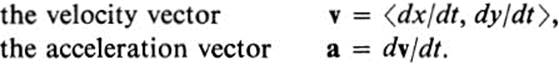
If the particle has mass m, then the kinetic energy of the particle at each point of the path C is defined by
![]()
Newton’s second law of motion states that at each point,
![]()
Using this notation, show the following.
a. The work done by the force F in moving the particle along the path C is equal to
![]()
b. At each point of the curve C, the rate of change of kinetic energy is given by
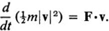
c. The kinetic energy of the particle at the end of the path C is equal to its kinetic energy at the beginning plus the total work done by the force in moving the particle along the path. (This is the work-energy principle.)
22.17 Let F = ![]() p, q
p, q ![]() be a conservative force field, and let f(x, y) be a potential function. The potential energy of a particle is defined at each point by
be a conservative force field, and let f(x, y) be a potential function. The potential energy of a particle is defined at each point by
![]()
where c is a constant that may be chosen in any convenient manner. (The value of c is not important, since it is always the difference in potential energy between two points that plays a role.)
a. Show that if the force F moves a particle along a path C, then the potential energy of the particle is decreased by the amount of work done by the force F.
(Note that the force required at each point to move the particle against the field would be − F. Thus the potential energy is increased by the amount of work done against the field. For example, lifting a weight against the force of gravity increases its potential energy. If the weight is allowed to drop, its potential energy decreases by the amount of work done by the gravitational field during the motion. These considerations explain why potential energy in physics is chosen to be the negative of the potential function in mathematics.)
b. Prove the law of conservation of energy : if a particle moves along a path C under the action of a conservative force field, then the sum of its potential energy and kinetic energy remains constant.
*22.18Let f(x, y) be continuous in a domain D. A natural question is whether there exists a solution g(x, y) of the equation
![]()
in D. According to Lemma 22.3, a solution always exists if D is a disk. Similarly, Lemma 22.4 guarantees that the equation
![]()
has a solution h(x, y), if D is a disk. However, these equations do not necessarily have solutions in an arbitrary domain D. Suppose for example, that we choose
![]()
Then f(x, y) is continuous in D (and in fact in the whole plane except for the point (0, 1), which is not in D, although it is a boundary point of D.). Show that there cannot exist a continuous function g(x, y) in D satisfying gx = f. (Hint: proceed by contradiction. Suppose there were such a function g(x, y). Then
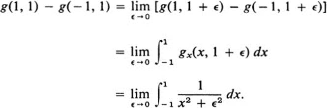
However, for fixed ![]() > 0 the latter integral can be evaluated explicitly, and it may be verified that
> 0 the latter integral can be evaluated explicitly, and it may be verified that
![]()
This contradiction proves the result.)
Remark The problem of finding a function f(x, y) that satisfies
![]()
for given p and q, arises in a variety of contexts and often under different names. In Ex. 22.17 it is the problem of finding the potential energy of a given force field. More generally, we have described it as the problem of finding a potential function of a given vector field. We note two more versions of the same problem.
First, using the notation of differentials (see the Remark following Ex. 16.16) the differential of a function f(x, y) is written as
![]()
Thus, if fx = p and fy = q, this may be written as
![]()
Starting with arbitrary functions p(x, y), q(x, y), the expression
![]()
is called a differential form (since it has the form of a differential of a function without necessarily being one). If there exists a function f(x, y) satisfying fx = p, fy = q, then p dx + q dy is called an exact differential form or an exact differential. Thus the problem of deciding whether a differential form p dx + q dy is exact, and if it is exact, of representing it as the differential of a given function, is precisely the same as deciding whether the vector field ![]() p, q
p, q ![]() is conservative, and if it is conservative, finding a potential function. Using the terminology of differentials, Th. 22.1 may be stated in the form
is conservative, and if it is conservative, finding a potential function. Using the terminology of differentials, Th. 22.1 may be stated in the form
![]()
If C joins (x1, y1) to (x2, y2), then the notation
![]()
is permissible whenever the integral is independent of path. Lemma 22.1 may then be stated as follows: if p dx + q dy is exact, and equal to df, then
![]()
Thus, the differential notation is highly suggestive. For the actual computation of the function f(x, y) from a given p and q, the method of Ex. 22.7 may be used.
As a final example of the same problem in a different context, consider the ordinary differential equation
![]()
A solution consists of a function y = g(x) such that
![]()
Such equations often arise in the form
![]()
in which case φ(x, y) = −p(x, y)/q(x, y). If the vector field ![]() p, q
p, q ![]() has a potential function f(x,y), then applying the implicit function theorem to a level curve f(x y) = c near a point where fy ≠ 0, we find that this level curve may be written as y = g(x), where
has a potential function f(x,y), then applying the implicit function theorem to a level curve f(x y) = c near a point where fy ≠ 0, we find that this level curve may be written as y = g(x), where
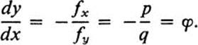
The level curves of f(x, y) are therefore implicit forms of solutions to the given equation. If such a function f exists, Eq. (22.15) is called an exact differential equation. Equation (22.15) is also often written in the form
![]()
using the notation of differentials. In fact, the following three statements are equivalent :
1. p(x, y) + q(x, y) dy/dx = 0 is an exact differential equation.
2. p dx + q dy is an exact differential form.
3. ![]() p, q
p, q ![]() is a conservative vector field.
is a conservative vector field.
Thus, solutions of an exact differential equation may be represented as level curves of a function f(x, y), where f(x, y) may be found explicitly by the method of Ex. 22.7.
We note in conclusion that multiplying through Eq. (22.15) by a nonzero function h(x, y) gives a new equation
![]()
where ![]() = hp,
= hp, ![]() = hq. The solutions of Eq. (22.16) coincide with those of Eq. (22.15) . (Equations (22.15) and (22.16) are in fact two forms of the same equation.) In particular, if Eq. (22.15) is not exact, it is of interest to look for a function h(x, y) that makes Eq. (22.16) exact, in which case solutions may be found by the method indicated above. Such a function h(x, y) is called an integrating factor for Eq. (22.15). Finding an integrating factor is equivalent in our terminology to making a given vector field conservative by changing its magnitude at each point (see Exs. 22.10 and 22.11). There is no general solution to the problem of finding an integrating factor, but there are methods for treating a variety of important special cases. These are discussed in detail in books on differential equations.
= hq. The solutions of Eq. (22.16) coincide with those of Eq. (22.15) . (Equations (22.15) and (22.16) are in fact two forms of the same equation.) In particular, if Eq. (22.15) is not exact, it is of interest to look for a function h(x, y) that makes Eq. (22.16) exact, in which case solutions may be found by the method indicated above. Such a function h(x, y) is called an integrating factor for Eq. (22.15). Finding an integrating factor is equivalent in our terminology to making a given vector field conservative by changing its magnitude at each point (see Exs. 22.10 and 22.11). There is no general solution to the problem of finding an integrating factor, but there are methods for treating a variety of important special cases. These are discussed in detail in books on differential equations.