Two-Dimensional Calculus (2011)

Chapter 4. Integration

24. The double integral

Having at our disposal a definition and the basic properties of area, we can now define the double integral. Our definition for an arbitrary figure is a natural extension of the one given at the beginning of the previous section for the case of a rectangle.

Let f(x, y) be a bounded function defined at all points of a figure F. Let F₁, …, F_n be an arbitrary partition of F, and form the sum

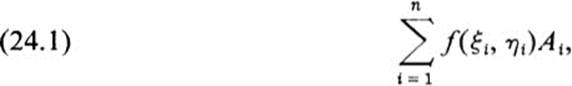
where (ξ_i, η_i) is any point of F_i, and A_i is the area of F_i. We wish to form the limit of this expression as the partition of F becomes finer and finer. To make this notion precise, we introduce the following terminology.

Definition 24.1 The diameter of a figure F is the maximum distance between two points of F

Definition 24.2 The norm of a partition F₁ . . ., F_n of a figure F is the maximum diameter of the figures F₁, …, F_n.

Definition 24.3 The expression (24.1) is said to tend to a limit l as the norm of the partition tends to zero if for every > 0 there exists a δ > 0 such that

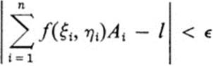
for every partition whose norm is less than δ.

Definition 24.4 If the expression (24.1) tends to a limit l as the norm of the partition tends to zero, then f(x,y) is said to be integrable over F, and the limit l is called the double integral of f over F and is denoted by

Before investigating properties of the double integral, let us give two interpretations in the case that f is a positive continuous function.

Geometric Interpretation: Volume

By a procedure exactly analogous to that used in the previous section for defining the area of a two-dimensional figure, we can define the notion of volume for a three-dimensional body and show that it has properties similar to those described in Ths. 23.1 and 23.3. In particular, the volume of a cylindrical body of constant cross section is equal to its height multiplied by the area of its base. Thus each term in the sum (24.1) represents the volume of the cylindrical body with base F_i and height f(ξ_i,η_i). This sum is therefore an approximation to the volume of the body lying over the figure F and under the surface z = f(x,y) (see Fig. 24.1). The precise volume of this body is obtained by taking finer and finer partitions of F and is thus equal to the limiting value of the sum (24.1), which is the double integral ∫ ∫_F f dA.

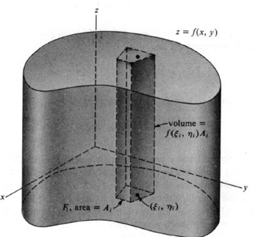
FIGURE 24.1 Volume under a surface

Physical Interpretation : Mass

If the figure F represents a thin plate of constant density c ( = mass per unit area), then the total mass of the plate is equal to cA, where A is the area of F. If a thin plate in the shape of the figure F has a variable density given by a function f(x, y), then each term in the sum (24.1) represents an approximation to the mass of the figure F_i ; namely, it represents the mass that the figure F_i would have if it had constant density equal to f(ξ_i, η_i). The total mass is therefore approximated by the sum (24.1), and it is precisely equal to the limiting value ∫ ∫_F f dA.

Just as in the case of the ordinary integral for functions of a single variable, one rarely applies the definition directly to compute the value of an integral. The definition is used to deduce certain basic properties, and from these properties are derived methods of computation. For the double integral, the basic properties are stated in the following theorem.

Theorem 24.1 The double integral has the following properties.

1. If f is integrable over F, and f ≥ 0, then ∫ ∫_F f dA ≥ 0.

2. If f and g are both integrable over F, and if λ, μ are any two constants, then λf + μg is also integrable over F, and

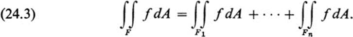
3. If F₁ ,…, F_n form a partition of F, and if f is integrable over F, then f is integrable over each F_i and

4. The function f ≡ 1 on F is integrable over F, and

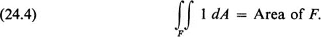
PROOF. Properties 1 and 2 are an immediate consequence of the fact that the corresponding properties hold for each of the partial sums of (24.1), and they must therefore continue to hold in the limit. We do not prove property 3 in detail, but we note that if each of the figures F₁,…, F_n is partitioned, then the combined figures of all the partitions form a partition of F. Using partitions of F formed in such a way yields Eq. (24.3). Finally, property 4 follows from the fact that for the function f ≡ 1, each of the partial sums(24.1) equals the area of F, by property 2 in Th. 23.1

We next show that these four properties serve to characterize uniquely the double integral.

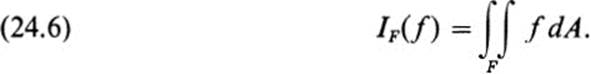
Theorem 24.2 Suppose that to each figure F and to each function f integrable over F there is assigned a number I_F(f), in such a way that the following conditions are verified.

1. If f ≥ 0 on F, then I_F(f) ≥ 0.

2. I_F(λf + μg) = λI_F(f) + μI_F(g), for any constants λ, μ.

3. If F₁,…, F_nform a partition of F, then

4. I_F(1) = area of F.

Then the following condition also holds:

and furthermore, for all F and f,

PROOF. To derive (24.5), note first that choosing λ = 1, μ = − 1 in condition 2 yields I_F(f − g) = I_F(f) − I_F(g). Now f ≥ g means f − g ≥ 0, and applying condition 1 to the function f − g gives I_F(f) − I_F(g) = I_F(f − g) ≥ 0, which proves (24.5). To prove (24.6), let F_u,…,F_n be any partition of F. Let A_i be the area of F_i and let,

Then

By condition 4, we have

and by condition 2,

By (24.5) and (24.7), we have

and, again using conditions 2 and 4,

Combining all these yields

If we sum over all F_i in the partition and use condition 3, we obtain

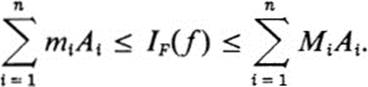
However, since both m_i and M_i represent the values of the function f at points of F_i, both the left- and right-hand sides of this inequality are sums of the form (24.1). By the definition of the integral, both sides tend in the limit to ∫ ∫_F f dA. Since the quantity I_F(f) is bounded above and below by quantities that converge to the same limit, it must equal this limit. This proves the theorem.

Remark 1 The significance of this theorem is that it reduces all properties of the double integral to four basic ones. The first property is known as positivity, and the second as linearity. These are basic properties of integration, and hold equally for ordinary integrals and line integrals. Some analog of property 3 is also common to all forms of integration. Property 4 is, of course, specially related to double integrals. Since many different definitions are possible for the double integral, it is important to know that as long as these four basic properties are satisfied, the value obtained from any alternative definition must coincide with ours.

Remark 2 It is useful to observe that the conclusion of the theorem continues to hold even if the quantity I_F(f) is not defined for all integrable f on F, but only for a subset. This subset must be large enough so that the statement of the properties makes sense. For example, the subset must include the function that is identically equal to 1 on any figure, and with each pair of f, g, it must include the linear combination λf + μg. An example of such a subset is the set of all continuous functions on each figure F. One can in fact prove that every function f continuous onF is integrable over F, but we do not give the proof here. If a number I_F(f) is assigned to each continuous f on F, in such a manner that the four given conditions are satisfied, then this number must coincide with the double integral. We see an example of how this may be done in Th. 24.3. Another useful class of functions are the piecewise continuousfunctions, obtained by “patching together” a number of functions, each of which is defined and continuous on one figure in a partition of F. Such functions are also integrable over F.

Remark 3 The proof of Th. 24.2 as it stands is valid only if the functions f are taken to be continuous, since we assumed that each function f had a maximum and minimum on each figure F₁. This is true of continuous functions, as we have noted in Th. 8.3. To prove Th. 24.2 for arbitrary integrable functions f would require an elaboration of the above argument.

The next theorem provides the method most often used for the actual computation of a double integral. Stating the theorem for an arbitrary figure F necessitates the introduction of some complex notation, which is apt to appear forbidding at first sight. It may be advisable to read through the theorem and its proof without concentrating on details, and then to study the subsequent remarks and examples. Familiarity with the way the theorem is applied in various cases greatly helps to clarify the general statement.

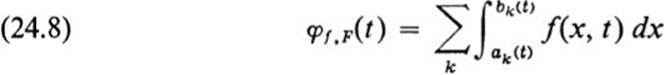
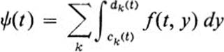
Theorem 24.3Let F be an arbitrary figure. Let c and d represent the minimum and maximum values of the y coordinate on F. For each value of t, c ≤ t ≤ d, the part of the line y = t lying in F consists of a number of intervals of the form a_k(t) ≤ x ≤ b_k(t) (see Fig. 24.2). Let f(x, y) be an integrable function on F, and suppose that the expression

exists for every t, c ≤ t ≤ d. Suppose further that the integral

exists. Then

PROOF. We must show that the quantity I_F(f) defined by (24.8) and (24.9) satisfies the conditions of Th. 24.2. We shall carry out the proof only for the case of polynomial figures. We note first of all that if F is a polynomial figure, then for each t there will be only a finite number of intervals a_k(t) ≤ x ≤ b_k(t).

Property 1. If f ≥ 0, then by (24.8) φ_{f, F}(t) ≥ 0 for all t, and by (24.9),I_F(f)≥ 0

Property 2. If h(x, y) = λ f(x, y)+ μg(x, y), then by (24.8), for c ≤ t ≤ d we have φ_h,Ft) = λφ_f,F(t) + μφ_g,F(t), and by (24.9), I_F(h) =λI_F(f) + μI_F(g).

Property 3. If F₁, …, F_n form a partition of F into polynomial figures, then for c ≤ t ≤ d we have φ_{f, F}(t) = φ_{f, F}(t)+…+φ _f, F_n(t), except for at most a finite number of values of t for which the line y = t contains a line

FIGURE 24.2 Notation for Th. 24.3

segment that is a common boundary of two different F_i. It follows from (24.9) that I_F(f) = I_F1(f) + … + I_Fn(f)

Property 4. If f ≡ 1, then for c ≤ t ≤ d, we have

in the notation of Th. 23.3. It follows from that theorem that

Thus the quantity I_F(f) satisfies the hypotheses of Th. 24.2, and Eq.(24.10) follows.

Remark 1 In the case that f(x, y) is continuous on F, the integrals (24.8) and (24.9) always exist, and (24.10) holds.

Remark 2Substituting the expression (24.8) for φ_f,F(t) in (24.9), we may write (24.10) in the form

where the limits of integration on the right are determined by the figure F in the way indicated in the theorem. The right-hand side of (24.11) is referred to as an iterated integral of a function of two variables. We first hold y fixed and integrate with respect to x, obtaining a number that depends on y. This gives us a function of y, which we then integrate with respect to y. The theorem states that this process of repeated ordinary integration yields the same value as the double integral.

Remark 3 Let f be a positive continuous function, and consider the three-dimensional body B lying above the figure F and under the surface z = f(x,y). The quantity φ_f,F(t), then represents the area of the section cut out of the body B by the vertical plane y = t (see Fig. 24.3). In view of our interpretation of the double integral as the volume of the body B, Th. 24.3 states that the volume may be obtained by integrating the cross-sectional area. This is the precise analog for volume of Th. 23.3 for area, which stated that area is equal to the integral of cross-sectional width.

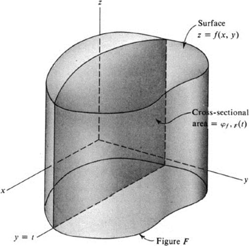
FIGURE 24.3 Cross-sectional area

Remark 4 When computing the integral of a given function f(x, y) over a given figure F we simplify the notation by omitting the subscripts f, F and writing φ(t) for φ_f,F(t).

Example 24.1

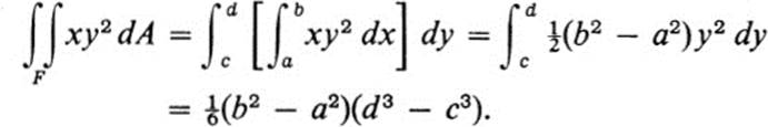
Let F be the rectangle a ≤ x ≤ b, c ≤ y ≤ d. Evaluate ∫ ∫_F xy² dA.

In this case each horizontal line y = t, c ≤t ≤ d,intersects F in the interval a≤ x ≤b. Thus, if f(x, y) = xy², then

and

RemarkIn the notation of (24.11), we would write

Example 24.2

Find the volume of the body lying above the square 0 ≤ x ≤ 1,0 ≤ y ≤ 1, and under the surface z = xy² ( Fig. 24.4).

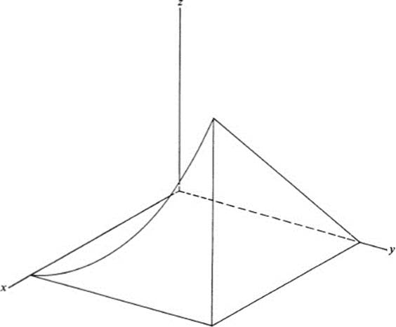
FIGURE 24.4 Volume under the surface z = xy², over a square

If F denotes the square indicated, then the volume is given by ∫ ∫_F xy² dA. We find its value simply by substituting a = 0, b = 1, c = 0, d = 1 in Example 24.1; the answer is

Example 24.3

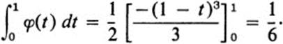
Find the volume of the right isosceles tetrahedron cut out of the first octant by the plane x + y + z = 1.

The volume in question is bounded above by the plane z = 1 − x − y and below by the triangle in the x, y plane described by x ≥ 0, y ≥ 0, x + y ≤ 1 ( Fig. 24.5). If we denote this triangle by F, then the volume is equal to ∫∫_F (1 ≤ x ≤ y) dA. For 0 ≤ t ≤ 1, the line y = t cuts F in the interval 0 ≤ x ≤ 1 − t. Thus

and

Example 24.4

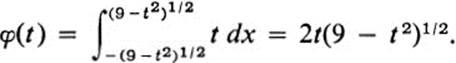
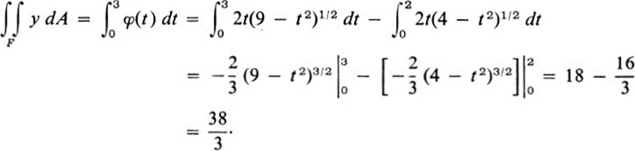
Evaluate ∫∫_F y dA, where F is defined by y ≥ 0, 4 ≤ x² + y² ≤ 9 ( Fig. 24.6).

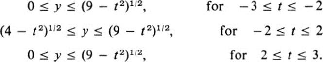
The line y = t intersects the figure F for those values of t satisfying 0 ≤ t ≤ 3. When 0 ≤ t < 2, the intersection consists of the two distinct segments

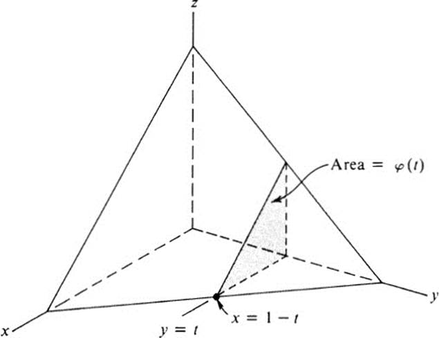
FIGURE 24.5 Volume of a tetrahedron

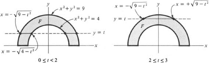
FIGURE 24.6 Integration over upper half-annulus

For 2 ≤ t ≤ 3, there is a single segment −(9 − t²)^1/2 ≤ x ≤ (9 − t²)^1/2 Thus, for 0 ≤ t ≤ 2,

while for 2 ≤ t ≤ 3,

Thus

We next state the theorem corresponding to Th. 24.3, with the roles of the x and y axes reversed.

Theorem 24.4 Let F be an arbitrary figure. Let a and b represent the minimum and maximum values of the x coordinate on F. For each value of t, a ≤ t ≤b, the part of the line x = t lying in F consists of a number of intervals of the form c_k(t) ≤ y ≤ d_k(t). Let f(x, y) be an integrable function on F, and suppose that the expression

exists for every t, a ≤ t ≤ b. Then

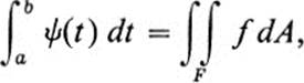
provided the integral on the left exists.

PROOF. Identical to that of the previous theorem.

Corollary In the notation of Ths. 24.3 and 24.4, we have

assuming that all the integrals in question exist; each side of (24.12) equals the double integral∫∫ _F f dA.

Remark Equation (24.12) may be written in the abbreviated form

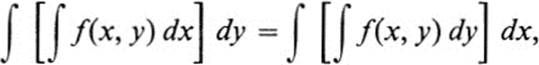
always bearing in mind that the limits of integration are determined by the particular figure. This equation asserts that the value of an iterated integral does not depend on the order of integration. It is sometimes referred to as Fubini’s theorem.

Example 24.5

Evaluate the integral in Example 24.4, using the method of Th. 24.4.

In this case, the line x = t intersects F for − 3 ≤ t ≤ 3, and the intersection consists of a single segment (see Fig. 24.7). This segment is

Thus

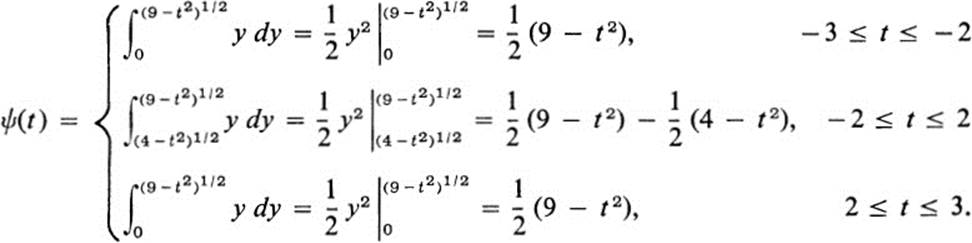
Finally

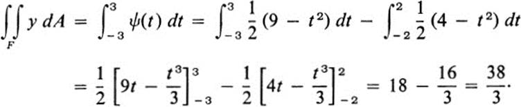
Thus, Eq. (24.12) is verified in this particular case.

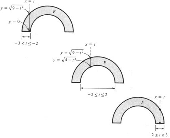
FIGURE 24.7 Integration over half annulus: alternative approach

Remark Once the procedure involved in evaluating an iterated integral is clearly understood, there is no need to introduce the auxiliary variable t. It is sufficient to consider one of the two variables to be fixed, and integrate with respect to the other, thus obtaining the expression inside the brackets on either side of (24.12). A second integration is then carried out with respect to the variable originally held fixed.

We conclude this section with a brief discussion of one of the many applications of double integration.

Definition 24.5 For an arbitrary figure F, the quantities

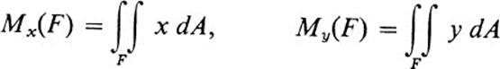
are called the moments of F with respect to the y and x axes, respectively.

The physical meaning of these quantities may be described as follows. Suppose that the figures F₁ and F₂ are cut out of cardboard and placed on opposite sides of a seesaw attached along the y axis ( Fig. 24.8). Then the side that goes down is the one whose figure has the greater x moment |M_x(F)| . The two sides balance if and only if the moments are equal in magnitude | M_x(F₁)| = | M_X(F₂)|. Since the x coordinate is positive on one side of the y axis and negative on the other side, the condition for balance may be written as M_x(F₂) = − M_x(F₁), or M_x(F₁) + M_x(F₂) = 0.

Suppose that a single figure F is placed so that it crosses the y axis, and we wish to know whether it will balance by itself. We may consider it to be divided by the y, axis into two figures, F₁ F₂, and according to the above discussion it balances if and only if M_x(F) = M_x(F₁) + M_x(F₂) = 0. A similar discussion applies to the y moment and balancing along the x axis.

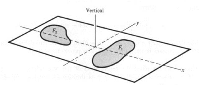
FIGURE 24.8 Moments and “balancing”

Definition 24.6 For any figure F, the point defined by

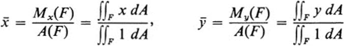
is called the centroid of F.

Lemma 24.1 The centroid of a figure is a point that depends only on the geometry of the figure, and not on the choice of coordinates ; more precisely, if new coordinates are chosen by a translation or rotation of the axes, and if the centroid is computed in these coordinates, then the point obtained is the same as in the original coordinates.

PROOF. Suppose first that new coordinates are chosen by a translation of the axes X = x −h, Y = y − k. Then

and

Similarly, = − k. Thus are the coordinates with respect to the new axes of the same point whose coordinates with respect to the original axes were ,

In particular, by making a preliminary translation of axes if necessary, we may assume that the centroid of Flies at the origin; that is, = (0, 0) or ∫∫_F x dA = ∫∫_F y dA = 0 (see Ex. 24.15). Suppose next that new coordinates are chosen by a rotation of axes X = x cos α − y sin α,Y = x sin y + y cos α. Then

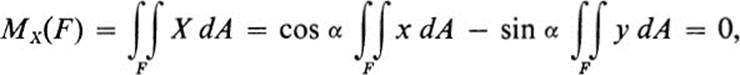
and similarly, M_Y(F) = 0. Thus = (0,0), and the centroid with respect to the rotated axes is again the origin. This proves the lemma.

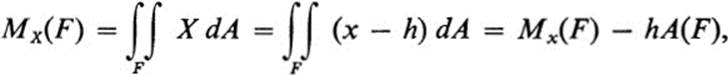
Concerning the physical interpretation of the centroid we note that if we choose a new Y axis to pass through the centroid, by setting X = x − then

so that the figure F balances about the Y axis (X = 0), which is to say, about the line x = Similarly, it balances about the line y = Thus, one consequence of the above lemma is the following statement (which may not seem obvious by physical intuition): “if an arbitrary figure balances about each of two perpendicular lines, then it balances about every line through their intersection.”

Example 24.6

Find the centroid of the figure F: y ≥ 0, 4 ≤ x² + y² ≤ 9.

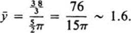
It is clear from the symmetry of F about the y axis, and may be verified directly, that M_x(F) = 0, and therefore = 0. In Example 24.4 we have computed for this figure M_y(F) = ∫∫_F y dA = The area A(F) is half of the area between two concentric circles of radius 2 and 3 ; thus A(F) = (9π − 4π) = Hence,

An interesting feature of this example is that it draws our attention to the fact that the centroid of a figure may well lie outside the figure itself (see Fig. 24.9).

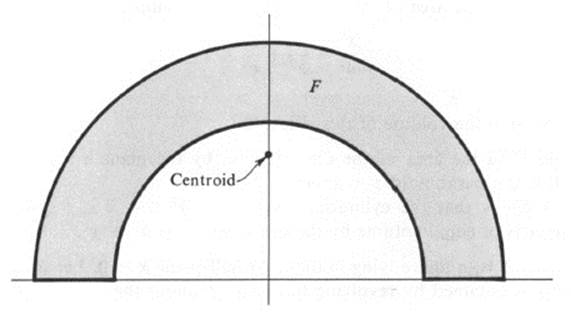
FIGURE 24.9 Centroid of a half annulus

Exercises

24.1Let F be the rectangle − 1 ≤ x ≤ 3, 2 ≤ y ≤ 5. Evaluate the following integrals.

a. ∫∫_F x²y dA

b. ∫∫_F (x² + y²) dA

c.

d. ∫∫_F xe^xy dA

24.2 Let F be the triangle x ≥ 0, y ≥ 0, x + 2y ≤ 1. Evaluate the following integrals.

a. ∫∫_F xy dA

b. ∫∫_F(x² + y²)dA

24.3 Let F be the disk x² + y² ≤ 4. Evaluate the following integrals.

a. ∫∫_F x²y dA

b. ∫∫_F(x² + y²)dA

*24.4 Let F be the trapezoid x ≥ 0, y ≥ 0, 1 ≤ x + y ≤ 2, and let f(x, y) = x + y.

a. Sketch F and find the function φ_f,F(t) of Eq. (24.8).

b. Find ∫∫_Ff dA.

24.5 Find the volume of the following three-dimensional bodies.

a. Lying over the square 0 ≤ λ: ≤ 1 and under the paraboloid z = x² y².

b. Lying under the surface z = xy and over the part of the disk x² + y² ≤ a² in the first quadrant.

c. The tetrahedron cut out of the first octant by the plane x/a + y/b + z/c = 1, a, b, c > 0.

In Exs. 24.6-24.8 use the fact that a three-dimensional volume is equal to the integral of its cross-sectional area.

24.6 a. Find the area of the cross section of the ellipsoid

with the plane y = t.

b. Find the volume of this ellipsoid.

24.7a. Find the area of the cross section by the plane z = t of the body bounded by the paraboloid z = x² + y².

b. Show that the cylindrical body x² + y²≤ 4, 0 ≤ z ≤ 4 is divided into two parts of equal volume by the paraboloid z = x²+ y².

24.8 Let F be a figure lying in the right half-plane x ≥ 0. Let B be the solid of revolution obtained by revolving the figure F about the y axis.

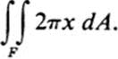
a. Show that the cross-sectional area of B with the plane y = t is given by the function φ_f,F (t) of Eq. (24.8), where f(x, y) = 2πx. (Hint: note that the cross section consists of a number of annular domains generated by the intervals a_k(t) ≤ x ≤ b_k(t).)

b. Show that the volume of B is equal to

24.9 Use the formula of Ex. 24.8b to find the volume of the following solids of revolution.

a. The ellipsoid x²/a² + y²/b² + z²/a² ≤ 1.

b. The torus obtained by revolving about the y axis the disk (x − b)² + y²≤ a², where b > a > 0.

c.The solid obtained by revolving about the y axis the figure 0 ≤ x≤ 1/y, 1 ≤ y ≤ b.

d. The limit of the volume obtained in part c as b → ∞.

24.10 a. Prove the Theorem of Pappus : If a figure F, which lies on one side of a line L, is revolved about the line L, then the volume of the resulting solid of revolution is equal to the area of F multiplied by the distance traveled by the centroid, that is,

where R is the distance from the centroid of F to the line L. (Hint: assume L is the y axis and use Ex. 24.8b.)

b. Use the theorem of Pappus to find the volume of the torus in Ex.24.9b.

c. Use the theorem of Pappus to find the centroid of the figure x²/a² + y²/b² ≤ 1, x ≥ 0. (Hint: use the result of Ex. 24.9a.)

*24.11 Prove that the centroid of an arbitrary triangle lies at the intersection of the medians. (Hint: one method would be to place the triangle so that a given median lies on the y axis, with the foot of the median at the origin. The vertices would then be (a, c), (0, b),(− a, −c). Show that the centroid then lies on the y axis.)

24.12 Let a figure F represent a thin ,plate of variable density ρ(x, y).The following physical quantities are represented in terms of double integrals.

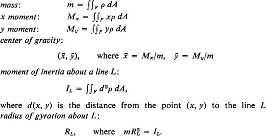
(Note: in case L is the y axis, we may use instead of I_L the notation I_x = ∫∫_F x²ρ dA ; if L is the x axis, we write I_y = ∫∫_F y²ρdA. If the density ρ(x, y) is constant, then the center of gravity coincides with the centroid of F, and the quantities _x, I_y are equal to the product of the density and ∫∫_F x² dA, ∫∫_F y² dA. These integrals are called the second x moment and second y moment of the figure F.)

a. Find the mass of the figure x² + y² ≤ a², y ≥ 0 if ρ(x, y) = y.

b. Find M_x for the figure x ≥ 0, y ≥ 0, x + y ≤ 1, if ρ(x, y) = x² + y²).

c. Find M_y for the figure 0 ≤ x ≤ a, 0 ≤ y ≤ b, if ρ(x, y) = x(x² + y²)^1/2.

d. Find M_x and M_y for the figure x² + y² ≤ a², x ≥ 0, y ≥ 0, where the density is proportional to the distance to the origin. (Hint: use Th. 24.3 or 24.4, depending on which is more convenient.)

e. Find the center of gravity of the half-disk of part a, where the density is proportional to the height above the x axis.

f. Find the center of gravity of the figure x² ≤ y, y² ≤ x if ρ(x, y) = ky.

g. Find the radius of gyration about the x axis of the figure in part f, with the given density.

h. Find the moment of inertia about the y axis of the figure x ≥ 0, y ≤ 2, 1 + x³ ≤ e^y, if ρ(x, y) = (1 + y³)/(1 + x³).

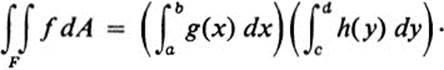
24.13 Let F be a rectangle a ≤ x ≤ b, c ≤ y ≤ d. Let f(x, y) = g(x)h(y). Show that

24.14 a. Let F be a figure that is symmetric about the y axis. Suppose that f(x, y) satisfies the condition f( − x, y) = −f(x, y). Show that ∫∫_F f dA = 0.

b. Show that if a figure F is symmetric about some straight line L, then the centroid of F lies on L.

24.15 Let P and Q be any two points in the plane. Show that an arbitrary rotation about the point P may be expressed as the composition of a translation taking P into Q, a rotation about Q and a translation taking Q back to P.

24.16 Let F be the rectangle a ≤ x ≤ b, c ≤ x ≤ d. Let h(x, y) ∈ in F, and let f(x, y) = h_xy(x, y). Show that

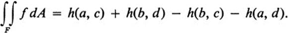
(Note the resemblance to the fundamental theorem of calculus for functions of a single variable.)

24.17 For each of the integrands f(x, y) in Ex. 24.1, find a function h(x, y) such that h_xy = f. Use Ex. 24.16 to check the answers to Ex. 24.1.

RemarkAt the end of Sect. 7, we considered ordinary integrals of a function of two variables with respect to one of the variables. A second integration with respect to the other variable yields an iterated integral, which may also be interpreted as a double integral, using Ths. 24.3 and 24.4. These relationships are the subject of Ex. 24.18-24.25.

24.18 Let f(x, y) be continuous in the triangle F:x ≤ b, y ≥ a, y ≤ x. Define

Show that

(Hint: show that both sides are equal to ∫∫_F f dA.)

24.19 Use the result of Ex. 24.18 to evaluate h(y) dy, where

24.20 Given a continuous function h of one variable, define a function g by

a. Show that g'(b) = h(y) dy,g˝(b) = h(b), and g(a) = g'(a) = 0.

b. Show that g(b) = (b − y)h(y) dy. (Hint: apply the method of Ex. 24.18.)

Note: the result of Ex. 24.20 may be stated as follows: if the indefinite integral h(t) dt of a function h is integrated again, the resulting function g can be expressed as a single integral. Using a somewhat ambiguous notation (whose meaning is made precise in Ex. 24.20) we may write this in the form

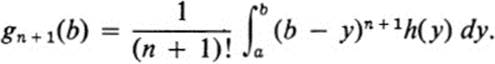
This process may be repeated. Denote the function g of Ex. 24.20 by g₁ and perform repeated indefinite integration; that is, define g_n by

(Again, using dubious notation, this could be written as

or in, more precise notation,

Then using induction and the reasoning of Ex. 24.20, it can be shown that g_n(x) may be expressed as a single integral,

See the following exercise; also compare with Ex. 7.23.

24.21Let

Show that

24.22 Certain figures may be expressed in both of the forms:

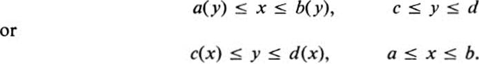
For example, the unit disk may be described by

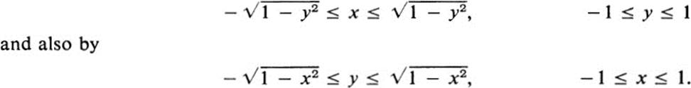
Each of the following figures is expressed in one of the above forms. Sketch the figure and express it in the other form.

a. 0 ≤ x ≤ 1 − y/2, 0 ≤ y ≤ 2

b.

c. x² ≤ y ≤ x, 0 ≤ x ≤ 1

d.

e.

24.23If F is a figure that can be represented in both of the forms given in Ex. 24.22, then the double integral over F of a function f(x, y) can be expressed in two ways as an iterated integral ; that is, by the Corollary to Th. 24.4, we have

This equation summarizes the method for change of order of integration, when two integrations are carried out successively. Namely, express the iterated integral as a double integral over some figure, and use that figure to express the double integral as an iterated integral in the other order.

Use this process to evaluate the following iterated integrals. Sketch the figure F in each case, expressing it in the two forms referred to in Ex. 24.22.

rl Γ λ(1-*²)^1/2 I

a.

b.

c.

d.

RemarkThe following section contains a number of important results that are based entirely on the equality of the iterated integrals

This is a special case of the Corollary to Th. 24.4. However, it is possible to give a direct proof in this case without using the theory of the double integral. Exercises 24.24 and 24.25 give two different methods of proof. The first one is a very simple argument that can be applied immediately in many cases. The second is more difficult, but also more direct, and applies to arbitrary continuous functions.

24.24Show that if there exists a function h(x, y) ∈ such that f(x, y) = h_xy(x, y), then (using the equality of the mixed derivatives h_xy, h_yx)

(Hint: compare with Ex. 24.16.)

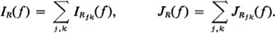
*24.25 Given a rectangle R:a ≤ x ≤ b, c ≤ x ≤ d, define

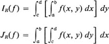
and A(R) = (b −a)(d − c) = area of R.

a. Show that if m ≤ .f(x, y) ≤ M on R, then

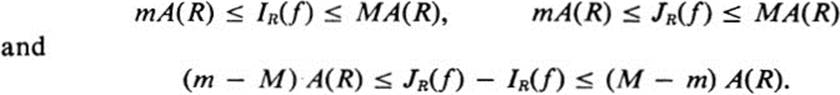
b. Show that if a rectangle R is divided into a number of smaller rectangles R_jk:X_j-1 ≤ x ≤ x_j, y_{k −1} ≤ y ≤ y_k by lines parallel to the x and y axes, then

c. Let f(x, y) be continuous on a rectangle R. Then f(x, y) is uniformly continuous on R (see the Remark following Lemma 7.2). This means that for any > 0, the rectangle R can be divided into sufficiently small rectangles R_jk such that the maximum M and minimum m of f on each R_jk satisfy M − m < . Using this fact, together with parts a and b above, show that for any > 0,

Deduce that J_R = I_R(f)

*24.26 Prove the following theorem: if f(x, y) is continuous on a figure F, if f(x, y) ≥ 0 at each point, and if ∫∫_F f dA = 0, then f(x, y) ≡ 0. (Hint: proceed by contradiction. If f(x₀,y₀) = η> 0 for some interior point (x₀, y₀) of F, then there exists an r > 0 such that f(x, y) > η/2 for (x − x₀)² + (y − y₀)² < r² (see Ex. 5.16a). It follows that ∫∫_F f dA ≥ πr²η/2 > 0. This shows that f(x, y) = 0 at every interior point of F. By continuity, f(x, y) = 0 at every boundary point of F.)

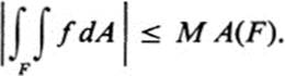
24.27 Show that if | f(x, y)| ≤ M on a figure F, and if the area of F is denoted by A(F), then

24.28 a. Show that if a figure F lies inside a rectangle R : a ≤ x ≤ b,c ≤ y ≤ d, then the centroid of F lies in R.

b. More generally, if F lies on one side of a line Ax + By + C = 0 then so does the centroid. (Hint: the hypothesis means that either Ax + By + C ≥ 0 or else Ax + By + C ≤ 0 throughout F.)

c. If F lies in a disk, so does the centroid of F. (Hint: if not, use part b to get a contradiction.)