Two-Dimensional Calculus (2011)
Chapter 4. Integration
26. Green’s theorem for arbitrary figures; applications
Our proof of Green’s theorem, which we gave for the special case of a rectangle, turns out to hold equally well for general figures. More precisely, the idea of the proof is unchanged, but the details must be modified.
Before discussing the general case, let us illustrate the argument for a specific figure (see also Ex. 25.14). Consider the figure
![]()
Let q(x, y) ∈![]() in a domain that includes F. We wish to evaluate ∫∫F qx dA. To do so, we use the method and notation of Th. 24.3. The horizontal line y = t intersects F for 0 ≤ t ≤ 3 ( Fig. 26.1). There are two cases to consider.
in a domain that includes F. We wish to evaluate ∫∫F qx dA. To do so, we use the method and notation of Th. 24.3. The horizontal line y = t intersects F for 0 ≤ t ≤ 3 ( Fig. 26.1). There are two cases to consider.
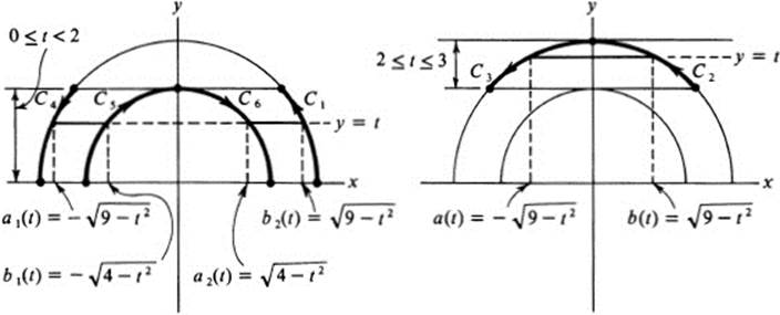
FIGURE 26.1 Proof of Green’s theorem for a semi-annulus
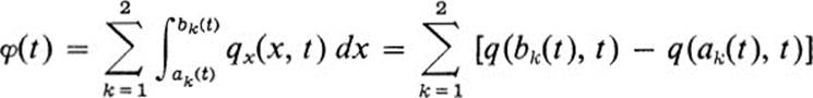
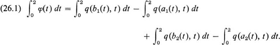
Case 1. 0 ≤ t < 2. The intersection of y = t with F consists of two line segments a1(t) ≤ x ≤ b1(t) and a2(t) ≤ x ≤ b2(t), where
Thus
and
We thus have four integrals each of which may be considered as a line integral along a part of the boundary of F. Consider, for example.
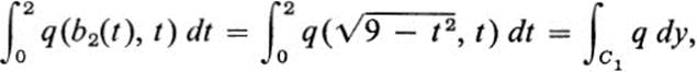
where the curve C1:x = ![]() y = t, 0 ≤ t ≤ 2, is an arc of the outer circle. Similarly,
y = t, 0 ≤ t ≤ 2, is an arc of the outer circle. Similarly,

where the curve ![]() :x =
:x = ![]() y = t, 0 ≤ t ≤ 2, is an arc of the inside boundary oriented in the direction of increasing y, and C6 is the same arc with the opposite orientation ( Fig. 26.1). Thus, with C4 and C5 denoting the (oriented) boundary arcs indicated in Fig. 26.1, Eq. (26.1) takes the form
y = t, 0 ≤ t ≤ 2, is an arc of the inside boundary oriented in the direction of increasing y, and C6 is the same arc with the opposite orientation ( Fig. 26.1). Thus, with C4 and C5 denoting the (oriented) boundary arcs indicated in Fig. 26.1, Eq. (26.1) takes the form

Case 2. 2 ≤ t ≤ 3. The intersection of y = t with F consists of a single segment. We have a(t) = −![]() b(dt) =
b(dt) = ![]()
![]()
and
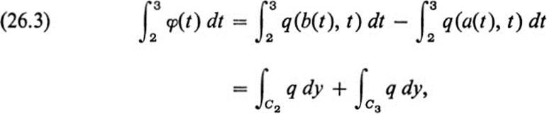
where C2 and C3 are the boundary arcs indicated in Fig. 26.1.
Let us denote by ![]() the entire outer semicircle of F, oriented in the counterclockwise direction, and let
the entire outer semicircle of F, oriented in the counterclockwise direction, and let ![]() denote the inner semicircle oriented in the clockwise direction ( Fig. 26.2). The curve
denote the inner semicircle oriented in the clockwise direction ( Fig. 26.2). The curve ![]() consists of the four arcs C1, C2, C3, C4, while
consists of the four arcs C1, C2, C3, C4, while ![]() consists of C5 and C6. Thus, adding Eqs. (26.2) and (26.3) , and applying Th. 24.3, we have
consists of C5 and C6. Thus, adding Eqs. (26.2) and (26.3) , and applying Th. 24.3, we have

Finally, let ![]() :x = t, y = 0, − 3 ≤ t ≤ −2, and
:x = t, y = 0, − 3 ≤ t ≤ −2, and ![]() :x = t, y = 0,2≤ t ≤ 3, denote the two horizontal line segments indicated in Fig. 26.2.
:x = t, y = 0,2≤ t ≤ 3, denote the two horizontal line segments indicated in Fig. 26.2.
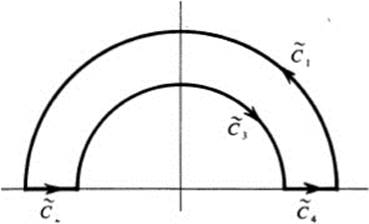
FIGURE 26.2 The oriented boundary of a semi-annulus
Then
and it follows from (26.4) that
where C is the piecewise smooth boundary curve of F, consisting of the successive arcs ![]() ,
,![]() ,
, ![]() ,
, ![]() . An analogous argument using Th 24.4 shows that
. An analogous argument using Th 24.4 shows that
for any function p(x, y)∈![]() in a domain that includes F. Equations (26.5) and (26.6), or their combined form
in a domain that includes F. Equations (26.5) and (26.6), or their combined form
constitute Green’s theorem for the figure F. Once the reasoning used in this special case is understood, there should be no difficulty in seeing how it extends to an arbitrary figure. In order to state the general theorem, it is useful to introduce the following notation.
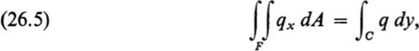
Definition 26.1 A curve C:x(t), y(t), a ≤ t ≤ b, lying on the boundary of a figure F is said to have positive orientation with respect to F if the vector ![]() − y'(t), x'(t)
− y'(t), x'(t) ![]() is directed toward the interior of F.
is directed toward the interior of F.
Remark The vector ![]() − y'(t), x'(t)
− y'(t), x'(t)![]() is perpendicular to the tangent vector
is perpendicular to the tangent vector ![]() x'(t),y'(t)
x'(t),y'(t)![]() obtained from the latter by a rotation through 90° in the counterclockwise direction. Thus, positive orientation with respect to F may be described as the direction of motion along C such that the interior of F lies to the left ( Fig. 26.3). Note that a figure F is typically bounded by one outer curve and a number of inner curves. Along the outer curve positive orientation means traversing the curve in the counterclockwise direction, whereas along the inner curves, positive orientation implies traversing in the clockwise direction.
obtained from the latter by a rotation through 90° in the counterclockwise direction. Thus, positive orientation with respect to F may be described as the direction of motion along C such that the interior of F lies to the left ( Fig. 26.3). Note that a figure F is typically bounded by one outer curve and a number of inner curves. Along the outer curve positive orientation means traversing the curve in the counterclockwise direction, whereas along the inner curves, positive orientation implies traversing in the clockwise direction.
FIGURE 26.3 Positive orientation of boundary curves
Definition 26.2 The oriented boundary of a figure F, denoted by ∂F, consists of the totality of boundary curves of F, each of them assigned a positive orientation with respect to F.
Remark The only context in which we use the oriented boundary is in forming a line integral ∫∂F p dx + q dy, where p and q are continuous functions on the boundary of F. Thus
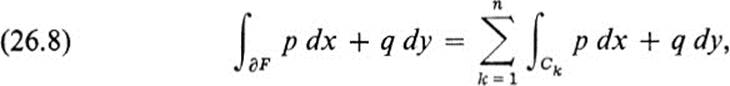
where the boundary of F consists of the curves C1 …, Cn, each assigned a positive orientation with respect to F. As we know from Lemma 21.1, the value of this integral does not depend on the parameter chosen to represent the curves Ck providing the orientation is preserved.
Example 26.1
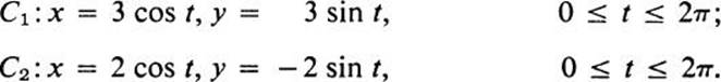
Evaluate ∫∂F y dx for the figure F:4 ≤ x2 + y2 ≤ 9.
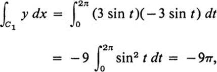
The boundary of F consists of two circles ( Fig. 26.4), which may be represented parametrically as
Note that along the outer curve C1 the vector
![]()
is directed toward the origin, hence toward the interior of F, while along the inner curve C2, the vector
![]()
is directed outwards, hence again toward the interior of F. Thus both C1 and C2 are positively oriented with respect to F. Now
and
![]()
thus
![]()
FIGURE 26.4 The positively oriented boundary of an annulus
Theorem 26.1 Green’s Theorem Let p(x,y), q(x, y) ∈![]() in a domain that includes a figure F. Then
in a domain that includes a figure F. Then

Remark Equation (26.9) is equivalent to the two separate equations

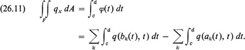
PROOF. We first evaluate ∫∫F qx dA, using the method and notation of Th. 24.3. Let us indicate the reasoning for the case where F is a polynomial figure.7 The line y = t intersects F in a finite number of intervals akt) ≤ x ≤ bk(t). We set
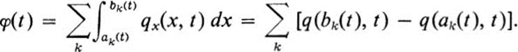
Then
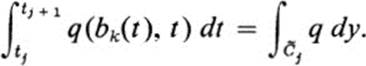
Now for each k, the integral ![]() (bkt), t) dt can be broken into a finite number of intervals such that in each interval, say tj ≤ t ≤ tj+1 the equations x = bk(t), y = t, define a curve
(bkt), t) dt can be broken into a finite number of intervals such that in each interval, say tj ≤ t ≤ tj+1 the equations x = bk(t), y = t, define a curve ![]() lying on the boundary of F. Then
lying on the boundary of F. Then
Since the point (bk(t), t) is a boundary point of F lying at the right-hand endpoint of a line segment contained in F, the interior of F lies to the left if ![]() is traversed in the direction of increasing y. Thus, each of the
is traversed in the direction of increasing y. Thus, each of the ![]() so defined is positively oriented with respect to F.
so defined is positively oriented with respect to F.
Similarly, each of the integrals ![]() qak(t), t) dt may be broken down into a sum, such that
qak(t), t) dt may be broken down into a sum, such that ![]() : x = ak(t), y = t, ti ≤ t ≤ ti + 1, is a curve on the boundary of F. Hence
: x = ak(t), y = t, ti ≤ t ≤ ti + 1, is a curve on the boundary of F. Hence
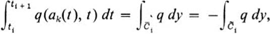
where ![]() consists of the curve
consists of the curve![]() with the opposite orientation. Since F lies to the right of
with the opposite orientation. Since F lies to the right of ![]() as
as ![]() is traversed in the direction of increasing y,
is traversed in the direction of increasing y, ![]() has negative orientation with respect to F, and
has negative orientation with respect to F, and ![]() therefore has positive orientation. If we form the sum over all k, the right-hand side of (26.11) represents a sum of line integrals of the form
therefore has positive orientation. If we form the sum over all k, the right-hand side of (26.11) represents a sum of line integrals of the form ![]() q dy, where each
q dy, where each ![]() is a curve lying on the boundary of F and having positive orientation with respect to F. Furthermore the totality of these
is a curve lying on the boundary of F and having positive orientation with respect to F. Furthermore the totality of these ![]() represents the complete oriented boundary of F, except for possible horizontal segments along which ∫q dy = 0. Thus, the right-hand side of (26.11) is equal to ∫∂F q dy, and (26.11) reduces to the first equation in (26.10). A similar reasoning using Th. 24.4 yields the second equation in (26.10). Combining these two equations, we obtain (26.9), and the theorem is proved.
represents the complete oriented boundary of F, except for possible horizontal segments along which ∫q dy = 0. Thus, the right-hand side of (26.11) is equal to ∫∂F q dy, and (26.11) reduces to the first equation in (26.10). A similar reasoning using Th. 24.4 yields the second equation in (26.10). Combining these two equations, we obtain (26.9), and the theorem is proved. ![]()
Example 26.2
Evaluate ∫∂F y dx for the figure F: 4 ≤ x2 + y2 ≤ 9.
We have already found the value −5π for this integral by a direct calculation. Using Green’s theorem, with p = y,q = 1, we find qx≡ 0, py ≡1, and
But the area of F is equal to the area inside a circle of radius 3 and outside a circle of radius 2; that is, 9π − 4π or 5π.
Example 26.3
Evaluate
![]()
where F is the square −1 ≤ x ≤ 1, −1 ≤ y ≤ 1.
In this case ∂F is a single closed curve C consisting of four line segments ( Fig. 26.5). We can find the value of (26.12) by computing the integral over each line segment and adding (see Ex. 25.6a). Green’s theorem cannot be applied directly, because the functions p, q in this case have a singularity at the origin. Thus the figure F, which contains the origin, does not lie in a domain where p(x, y), q(x, y)∈![]() We can, however, simplify the computation greatly by using the figure
We can, however, simplify the computation greatly by using the figure
![]()
where r is any fixed number between 0 and 1 ( Fig. 26.5). The boundary of F consists of two parts. The outer curve is the same as the boundary of F, and the inner curve is a circle of radius r. The functions p = −y/(x2 + y2), q = x/(x2+ y2) ∈![]() in the domain D consisting of the whole plane except for the origin. Since the figure
in the domain D consisting of the whole plane except for the origin. Since the figure![]() lies in this domain we may apply Green’s theorem. As we have observed before, qx − py ≡ 0 in this case, and therefore
lies in this domain we may apply Green’s theorem. As we have observed before, qx − py ≡ 0 in this case, and therefore
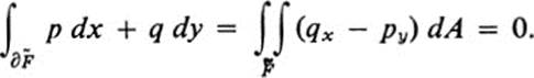
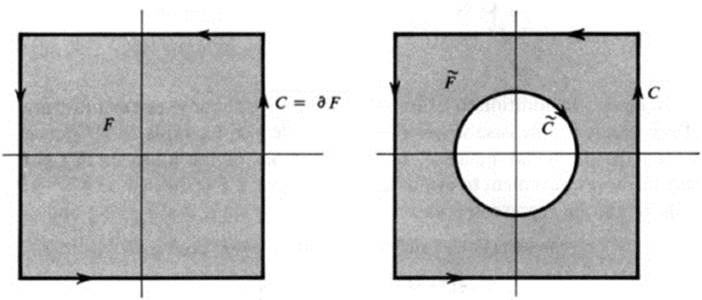
FIGURE 26.5 Use of Green’s theorem to reduce integral over a square to an integral over a circle
Denoting by C the inner circle, x = r cos t, y = — r sin t, 0 < t < 2π, positively- oriented with respect to F, and once again C = ∂F, we obtain
![]()
or
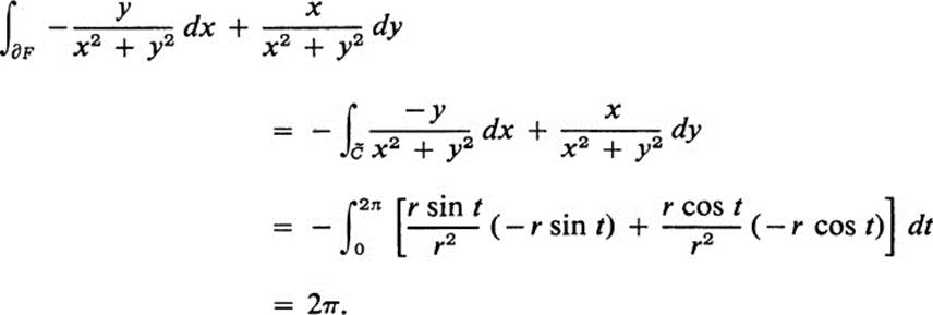
Thus we have found the integral in question, not by a direct integration over the original curve, but by reducing it to an integral over a simpler curve by virtue of Green’s theorem.
The above examples illustrate two of the many applications of Green’s theorem. We next consider the way in which Example 26.2 generalizes to arbitrary figures.
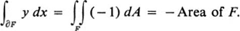
Lemma 26.1 Let F be an arbitrary figure, and A(F) its area; then

PROOF. Applying Green’s theorem to each of the boundary integrals on the right yields ∫∫F 1 dA = A(F). ![]()
Remark In addition to Example 26.2, we have already seen an illustration of this result for the case where F is a rectangle (see Example 25.1). Depending on the particular figure F, one or the other of the integrals in (26.13) may be more convenient to evaluate. For example, if F is the disk x2 + y2 ≤ r2, then ∂F can be represented as x = r cos t, y = r sin t, 0 ≤ t ≤ 2π, and
Each of these expressions integrated from 0 to 2π yields the value πr2, but the last one is clearly the simplest.
We are now able to prove a theorem that provides a basic link between the double integral and the theory of differentiable transformations. The Jacobian of a transformation, which first appeared as the determinant of an associated linear transformation, turns up here in a totally different manner.
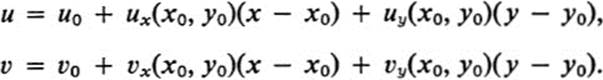
Theorem 26.2 Let u(x, y), υ(x, y) define a diffeomorphism G of a domain D onto a domain ![]() . Let F be a figure lying in D, and let its image be a figure
. Let F be a figure lying in D, and let its image be a figure ![]() ; then
; then
PROOF. We apply Lemma 26.1 to the figure ![]() . For this purpose, let us denote by C1 …, Cn the oriented curves which constitute ∂F. Let
. For this purpose, let us denote by C1 …, Cn the oriented curves which constitute ∂F. Let
![]()
be any one of these curves, and let
![]()
be its image under the transformation G. Using the chain rule we may transform any line integral over ![]() into a line integral over Ck. In particular,
into a line integral over Ck. In particular,
Now setting p = uυx, q = uυy we find
![]()
and
Applying Green’s formula (26.9) to the figure F, we find
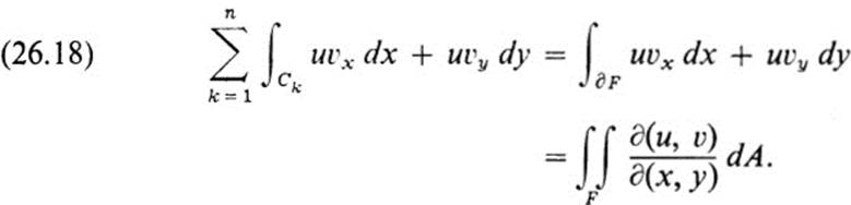
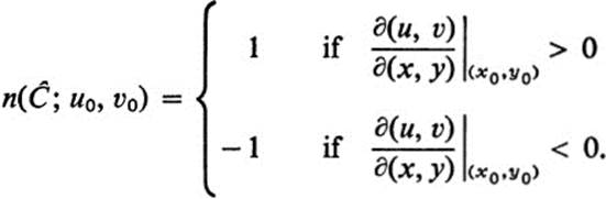
As we have remarked in the proof of Th. 18.2, for a diffeomorphism, the Jacobian is either everywhere positive or everywhere negative. If the Jacobian is positive, then the transformation G preserves orientation. This implies that since the figure F lies to the left when Ck is traversed in the direction of increasing t, the figure ![]() also lies to the left when
also lies to the left when ![]() is traversed in the direction of increasing t. In other words, for positive Jacobian, the fact that the curve Ck defined by (26.15) is positively oriented with respect to F implies that the curve
is traversed in the direction of increasing t. In other words, for positive Jacobian, the fact that the curve Ck defined by (26.15) is positively oriented with respect to F implies that the curve ![]() defined by (26.16) is positively oriented with respect to
defined by (26.16) is positively oriented with respect to ![]() . Thus the curves
. Thus the curves ![]() . . .,
. . ., ![]() constitute ∂
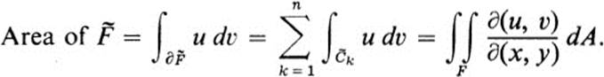
constitute ∂![]() . Applying Lemma 26.1 to F and using Eqs. (26.17) and (26.18) yields
. Applying Lemma 26.1 to F and using Eqs. (26.17) and (26.18) yields
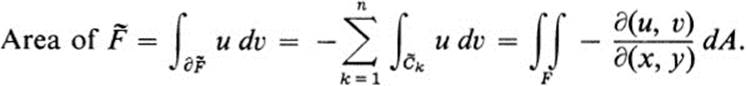
This proves (26.14) for the case that ∂(u, υ)/∂(x, y) > 0. In the opposite case, where ∂(u, υ)/∂(x, y) < 0, orientation is reversed, so that the curves ![]() defined by (26.16) are negatively oriented with respect to
defined by (26.16) are negatively oriented with respect to ![]() . In this case
. In this case
Since
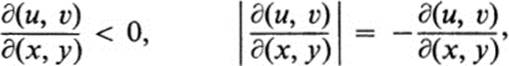
and (26.14) holds again. ![]()
Corollary Let
be a nonsingular linear transformation, and let Δ = det G = ad − bc. Then, if F is any figure in the x, y plane and ![]() is its image in the u, υ plane,
is its image in the u, υ plane,
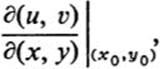
PROOF. Since a nonsingular linear transformation is a diffeomorphism of the whole x, y plane onto the u, υ plane, we may apply the theorem. But ∂(u, υ)/ ∂(x, y) = Δ, a constant, and (26.14) reduces to

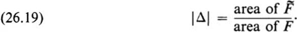
Remark We have already indicated the geometric interpretation on (26.19) of the determinant in Sect. 14, for the case where F was a disk, and at the end of Sect. 15, for the case where F was a triangle. One way to make Eq.(26.14) plausible is to note that the integral on the right-hand side is the limit of sums of the form
taken over partitions of F. If a figure Fi in the partition is taken to be a small triangle, then the differential of G at the point (ξi ηi) is a linear transformation that approximates G on Fi and whose determinant is equal to
Thus the corresponding term in the sum (26.20) equals the area of the image under the differential of G at (ξi ηi) and is approximately equal to the area of the image under G. Summing over i, we obtain a quantity that approximates the area of the image of all of F and Eq. (26.14) states that the sums (26.20) tend precisely to this area in the limit.
Example 26.4
Let G be the transformation
Let F be the figure x: ≥ 0, y ≥ 0, x2 + y2 ≤ 1.
To compute the integral in (26.14), we note
![]()
and
Thus

But

and we find (for example, by the trignometric substitution y = sin t):
![]()
Thus

Let us now examine the figure F and its image ![]() under the transformation G ( Fig. 26.6). Introducing polar coordinates
under the transformation G ( Fig. 26.6). Introducing polar coordinates
we find that G takes the form
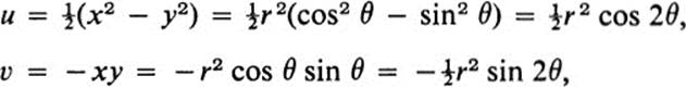
or
![]()
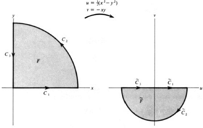
FIGURE 26.6 The image of a quarter disk under the transformation G:u = ![]() (x2 − y2), υ = −xy
(x2 − y2), υ = −xy
Thus each radius θ = θ0, 0 ≤ r ≤ 1, of the quarter circle F maps one-to-one onto the ray φ = − 2θ0, 0 ≤ R ≤ ![]() and the figure F maps one-to-one onto the semicircle
and the figure F maps one-to-one onto the semicircle ![]() : − π ≤ φ ≤ 0, 0 ≤ R ≤
: − π ≤ φ ≤ 0, 0 ≤ R ≤ ![]() . The area of
. The area of ![]() is =
is = ![]() π(
π(![]() )2 =
)2 = ![]() . which, in view of (26.21), confirms Eq. (26.14) for this example.
. which, in view of (26.21), confirms Eq. (26.14) for this example.
In conclusion, let us examine ∂F and ∂![]() . First of all, ∂F consists of a single closed piecewise smooth curve, obtained by describing in succession the following parts:
. First of all, ∂F consists of a single closed piecewise smooth curve, obtained by describing in succession the following parts:
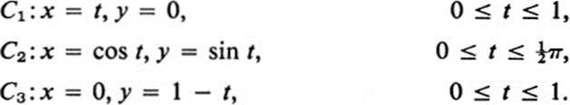
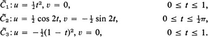
Their images under G are, respectively,
Thus ![]() and
and ![]() are each segments of the x axis, traversed from left to right, and
are each segments of the x axis, traversed from left to right, and ![]() is a semicircle traversed in the clockwise direction (see Fig. 26.6). We observe that C1, C2, C3 are positively oriented with respect to F, but
is a semicircle traversed in the clockwise direction (see Fig. 26.6). We observe that C1, C2, C3 are positively oriented with respect to F, but ![]() ,
,![]() ,
,![]() ,
,![]() are negatively oriented with respect to F. This reflects the fact that the transformation G has negative Jacobian, −(x2 + y2). Thus ∂F is the closed curve consisting of the three parts
are negatively oriented with respect to F. This reflects the fact that the transformation G has negative Jacobian, −(x2 + y2). Thus ∂F is the closed curve consisting of the three parts ![]() ,
,![]() ,
,![]() traversed in the opposite direction.
traversed in the opposite direction.
Exercises
26.1 Let C be the curve x = a cos t, y = b sin t, 0 ≤ t ≤ 2π. Use Green’s theorem to evaluate each of the following integrals.
a. ∫c y2ex dx
b. ∫c y cos x dx + (cos y + sin x) dy
c.![]()
d. ∫c y dx − x dy
26.2 Sketch each of the following figures F, and express in parametric form the curve or curves that constitute the oriented boundary ∂F.
a. ![]()
b. ![]()
c. F: 2x ≤ x2 + y2 ≤ 9
d. F: x2 ≤ y ≤ x1/2
e. F: y2 ≤ x ≤ 1
f. F: x + y ≤ 1, x − y ≥ − 1, y ≥ 0
26.3 Use Green’s theorem to evaluate
![]()
for each of the figures F in Ex. 26.2.
26.4 Use Lemma 26.1 to compute the area of the figures bounded by the following curves.
a. The ellipse x = a cos t, y = b sin t, 0 ≤ t ≤ 2π.
b. The astroid x = a cos3 t, y = a sin3 t, 0 ≤ t ≤ 2π.
c. The loop of the strophoid
![]()
(Hint: note that y = tx, and use the last expression in (26.13).)
d. The loop of the folium of Descartes
![]()
(Hint: use the same method as in part c. The resulting integral is an “improper integral” and is evaluated as a limit. See the discussion immediately following Eq. (28.12).)
e. The cardioid r = a(1 − cos θ), 0 ≤ θ ≤ 2π, where r and θ are polar coordinates. (Hint: see Ex. 21.25a.)
f. One “leaf” of the “rose” r = a sin 2θ, 0 ≤ 0 ≤ ![]() π. (Hint: see part e.)
π. (Hint: see part e.)
26.5 Let f(x) be a positive continuously differentiable function defined for a ≤ x ≤ b. Let F be the figure defined by
![]()
a. Show that if p(x, y) is continuous on the boundary of F, then
![]()
b. Using part a and Lemma 26.1, show that the area of F is equal to
![]()
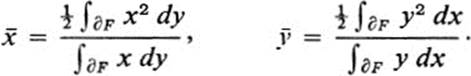
26.6Show that the centroid ![]() of a figure F is given by
of a figure F is given by
26.7 For each of the following figures F and transformations G, sketch ![]() and its image Funder G, and verify Eq. (26.14).
and its image Funder G, and verify Eq. (26.14).
a. F: x ≥ 0, x2 + y2 ≤ 1 ; G : u = x2, υ = y
b. F: −3 ≤ x ≤ −2, 1 ≤ y ≤ 2; G: u = x2, υ = y3
c. F:0 < a ≤ x ≤ b, 0 ≤ y ≤ π; G:u = x cos y, υ = x sin y
d. F:a ≤ x ≤ b, 0 ≤ y ≤ π; G:u = ex cos y, υ = ex sin y
26.8 Let C: x(t), y(t), a ≤ t ≤ b, be a regular curve lying on the boundary of a figure F, and suppose that C has positive orientation with respect to F. Show that at each point of C,
![]()
where s is the parameter of arc length along C, and N is the unit vector perpendicular to C directed toward the exterior of F.
26.9Let u(x, y) ≡![]() and υ(x, y) ≡
and υ(x, y) ≡![]() in a domain D. Let F be a figure lying in D. At each boundary point of F where the boundary curve is regular, define the normal derivative ∂υ∂n to be the directional derivative of υ(x, y) in the direction of the unit normal N directed toward the exterior of F. Prove the following identities.
in a domain D. Let F be a figure lying in D. At each boundary point of F where the boundary curve is regular, define the normal derivative ∂υ∂n to be the directional derivative of υ(x, y) in the direction of the unit normal N directed toward the exterior of F. Prove the following identities.
*a.![]()
Hint: apply Green’s theorem with p = − uυy, q = uvx and use Ex. 26.8.)
b. ![]()
c. ![]()
(Note: parts a and b are known as Green's identities.)
26.10Using the notation of Ex. 26.9, show that the following statements hold.
a. If υ(x, y) is harmonic in D, and if u(x, y) is equal to zero at each point of the boundary of F, then
b. If u(x, y) is harmonic in D, then
![]()
(Note: if u(x, y) represents temperature, then ∂u/∂n describes the rate of flow of heat across the boundary at each point. The integral ∫∂ F (∂u/∂n) ds represents the total flow across the boundary. The vanishing of this integral means that the total flow across the boundary is zero, or that the amount of heat entering the figure F is equal to the amount leaving F.)
26.11 Suppose u(x, y) is harmonic in a domain D. Setting υ(x, y) = u(x, y) in Green’s identity, Ex. 26.9a, yields
By Ex. 24.26, if the integral on the left is equal to zero, then ∇u ≡ 0 on F. Use this fact to prove the following statements.
a. If u(x, y) = 0 at each point of the boundary of F, then u(x, y) ≡ 0 in F. (See Corollary 3 to Th. 12.3 for a different proof.)
b. If ∂u/∂n = 0 at each point of the boundary of F, then u(x, y) is constant on F.
c. If u(x, y) and υ(x, y) are both harmonic in D, and if ∂u/∂n = ∂υ/∂n at each point of the boundary of F, then u(x, y) and υ(x, y) differ by a constant.
d. Suppose u(x, y) and υ(x, y) both satisfy Poisson's equation in D :
![]()
where f(x, y) is a given function. If u(x,, y) = vυ(x, y) at each point of the boundary of F, then u(x, y) ≡ υ(x, y) in F.
*26.12 Let h(x, y) ∈![]() in a domain D. Suppose that the disk
in a domain D. Suppose that the disk
![]()
lies in D. The quantity
![]()
is called the mean value of h(x, y) on the circle (x, − x0)2 + ( y − y0)2 = r2. (See the general discussion of mean values at the beginning of Sect. 27.) Using Ex. 26.9c and Lemma 7.2, one can prove the following relation
Carry out the details by verifying each step in the following string of equalities. Set
![]()
so that
![]()
then
26.13 Using the result of Ex. 26.12, prove the following theorem, known as the mean-value property of harmonic functions : if h(x, y) is harmonic in a domain D, then for every point (x0 y0) in D,
![]()
for every value of r such that the disk (x − x0)2 + (y − y0)≤ r2 lies in D.
(Hint: in the notation of Ex. 26.12, if h(x, y) is harmonic, then d/dr m(r) = 0, and m(r) is constant. But as a consequence of Lemma 7.2, m(r) is a continuous function of r, and limr→0 m(r) = m(0) = h(x0, y0).)
*26.14 The mean-value property described in Ex. 26.13 is a property unique to harmonic functions. This may be stated in the following manner: if h(x, y)∈![]() in a domain D, and if for every point (x0, y0) in D the value of h at(x0, y0) equals its mean value over all small circles about (x0y), then h(x, y) is harmonic in D.
in a domain D, and if for every point (x0, y0) in D the value of h at(x0, y0) equals its mean value over all small circles about (x0y), then h(x, y) is harmonic in D.
Prove this statement. (Hint: proceed by contradiction. Suppose that at some point (x0, y0) in D, Δh ≠ 0 say Δh(x0, y0) = η > 0. Then for some r > 0, Δh ≥ η/2 > 0 for (x − x0)2 + (y − y0)2≤ r2. By Ex. 26.12, m'(r) > 0. This contradicts the assumption m(r) = h(x0, y0).)
*26.15 Let h(x, y) be continuous on the circle C:(x− x0)2 + (y − y0)2 = r2, and suppose h(x, y) ≤ M on C. Show that if the mean value of h(x, y) on C is equal to M, then h(x, y) ≡ M on C. (Hint: let
![]()
and let f(r, θ) = M − g(r, θ). Then f(r, θ) is continuous for 0 ≤ θ ≤ 2π, and f(r, θ) ≥ 0. To show that ![]() f(r, θ) dθ = 0 implies f(r, θ) ≡ 0, proceed by contradiction. If f(r, θ0) = η > 0, then f(r, θ) ≥ η/2 for |θ − θ0| < δ, and
f(r, θ) dθ = 0 implies f(r, θ) ≡ 0, proceed by contradiction. If f(r, θ0) = η > 0, then f(r, θ) ≥ η/2 for |θ − θ0| < δ, and
![]()
26.16 Prove the strong maximum principle for harmonic functions : if h(x, y) is harmonic in a domain D, if h(x, y) ≤ M throughout D, and if h(x0, y0) = M for some point (x0, y0) in D, then h(x, y) ≡ M in D. Proceed in two steps.
a. Show that if h(x, y) has a local maximum M at (x0, y0) then h(x, y) ≡ M on every small circle about (x0, y0). (Hint: use Ex. 26.15 together with the mean value property of harmonic functions.)
*b. Show that if there were some point (x1, y1) in D such that h(x1, y1) < M, this would lead to a contradiction as follows. Join (x0, y0) to (x1, y1) by a curve C:x(t), y(t), 0 ≤ t ≤ 1 . Then the function hc(t) satisfies hc(0) = M, hc(l) < M. Let b be the largest value of t such that hc(b) = M. Then 0 ≤ b < 1, and applying part a to the point (x2, y2) = (x(b), y(b)) leads to a contradiction.
26.17 Let f(x, y)∈![]() in a domain D, and let
in a domain D, and let ![]() p, q
p, q ![]() = ∇f. Give two different proofs that for every figure F lying in D, ∫∂F p dx + q dy = 0.
= ∇f. Give two different proofs that for every figure F lying in D, ∫∂F p dx + q dy = 0.
26.18 Let f(x, y) ∈![]() in a domain D, except at a point (x0, y0). Let C1, C2 be circles in D defined by
in a domain D, except at a point (x0, y0). Let C1, C2 be circles in D defined by
![]()
Suppose that all points between these two circles also lie in D. Show that if Py = qx at every point of D except (x0, y0), then
![]()
(Hint: apply Green’s theorem to the figiire F bounded by Cx and C2. Pay careful attention to the orientation of ∂F and of Cx, C2.)
26.19 Under the same hypotheses as Ex. 26.18, let F be a figure lying in D. Show that the following statements hold.
a. If (x0, y0) does not lie in F, then ∫∂F p dx + q dy = 0.
b. If (x0 y0) is an interior point of F, then
![]()
where rx is chosen sufficiently small so that the set of points (x, y) satisfying (x − x0)2 +(y− y0)2 ≤ r2 lies in the interior of F. (Hint: apply Green’s theorem to the figure ![]() bounded by ∂F and C1.)
bounded by ∂F and C1.)
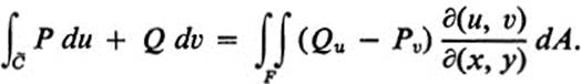
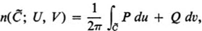
26.20 Let C be a piecewise smooth curve that forms the oriented boundary of a figure F. Show that the winding number n(C; >x0, y>0) of C about the point (x0, y0) satisfies

(Hint: see Ex. 25.18 for the definition of winding number, and use Ex. 26.19.)
26.21 Let G be a differentiable transformation of a domain D in the x, y plane into a domain E of the u, υ plane. Suppose P(u, υ),Q(u,υ)∈![]() in E. Set
in E. Set
![]()
and
![]()
Let C be a curve in D, and let ![]() be its image under G. Show that
be its image under G. Show that
![]()
(Note that Eq. (26.17) is a special case of this formula. Use the same reasoning here as was used to derive (26.17).)
26.22 Using the notation of Ex. 26.21, show that if C = ∂F, where F is a figure lying in D, then
(Hint: see Ex. 17.15a.)
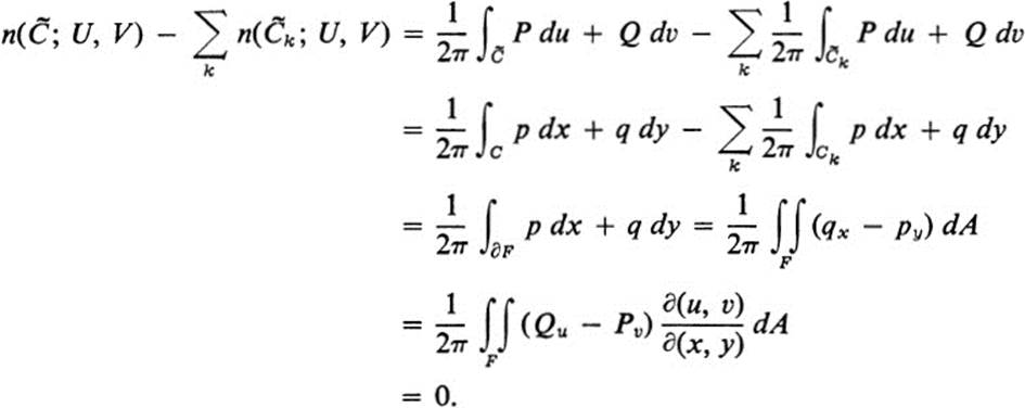
26.23 Using the notation of Ex. 26.21, let (x0, y0) be a point of D, and let F be the figure (x − x0)2 + (y − y0)2 ≤ r2, where r is chosen sufficiently small so that Flies in D. Let C = ∂F, and let ![]() be the image of C under the transformation G. Let (U, V) be any point in the u, υ plane such that G(x, y) ≠ (U, V) for all points(x, y) in F (that is, (U, V) is a point that is not in the image of the figure F). Show that the winding number n(
be the image of C under the transformation G. Let (U, V) be any point in the u, υ plane such that G(x, y) ≠ (U, V) for all points(x, y) in F (that is, (U, V) is a point that is not in the image of the figure F). Show that the winding number n(![]() ; U, V) = 0. (Hint: let
; U, V) = 0. (Hint: let
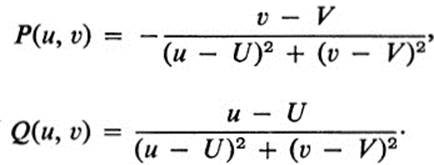
Then P(u, υ)∈![]() 1, Q(u, υ) ∈
1, Q(u, υ) ∈![]() in the domain E consisting of the whole plane minus the point (U, V), and Pυ = Qu in E. Since
in the domain E consisting of the whole plane minus the point (U, V), and Pυ = Qu in E. Since
the result follows from Ex. 26.22.)
Remark Ex. 26.23 gives a useful criterion for determining when a pair of equations
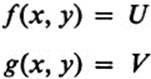
can be solved for x and y, when U and V are given. Namely, suppose C is a circle in the x, y plane, and ![]() is the image of C under the transformation
is the image of C under the transformation
![]()
If ![]() does not pass through the point (U, V) and if the winding number of
does not pass through the point (U, V) and if the winding number of ![]() about the point ( U, V) is different from zero, then the above equations must be satisfied by some point (x, y) lying inside C (since otherwise we could conclude from Ex. 26.23 that the winding number of
about the point ( U, V) is different from zero, then the above equations must be satisfied by some point (x, y) lying inside C (since otherwise we could conclude from Ex. 26.23 that the winding number of ![]() about (U, V) must equal zero). Exercise 26.24 shows how this reasoning may be used to guarantee the existence of a solution to a pair of simultaneous quadratic equations. It may be difficult to solve such a pair of equations explicitly, or even to determine whether a solution exists, since the equation may represent two ellipses, or an ellipse and a hyperbola, which may or may not intersect. In Ex. 26.28the same reasoning is used to prove a part of the inverse mapping theorem, which may be thought of as guaranteeing the existence of a solution of a pair of simultaneous equations. Exercise 26.29 completes the proof of the inverse mapping theorem. Exercises 26.25-26.27 lead up to this result, but they are also of interest in their own right for an understanding of some of the more subtle properties of differentiable mappings.
about (U, V) must equal zero). Exercise 26.24 shows how this reasoning may be used to guarantee the existence of a solution to a pair of simultaneous quadratic equations. It may be difficult to solve such a pair of equations explicitly, or even to determine whether a solution exists, since the equation may represent two ellipses, or an ellipse and a hyperbola, which may or may not intersect. In Ex. 26.28the same reasoning is used to prove a part of the inverse mapping theorem, which may be thought of as guaranteeing the existence of a solution of a pair of simultaneous equations. Exercise 26.29 completes the proof of the inverse mapping theorem. Exercises 26.25-26.27 lead up to this result, but they are also of interest in their own right for an understanding of some of the more subtle properties of differentiable mappings.
26.24 Let G be the mapping
Let ![]() be the image of the unit circle C :x = cos t, y = sin t, 0 ≤ t ≤ 2π.
be the image of the unit circle C :x = cos t, y = sin t, 0 ≤ t ≤ 2π.
a. Show that ![]() may be written in the form
may be written in the form
![]()
b. Show that n(![]() ; 2, 3) = 2.
; 2, 3) = 2.
c. Deduce that the equations
have a simultaneous solution (x, y) satisfying x2 + y2 < 1 .(Hint: use the reasoning indicated in the Remark just above.)
26.25 Let G be a linear transformation with determinant Δ ≠ 0. Let C be a circle x = r cos t, y = r sin t, 0 ≤ t ≤ 2π, and let ![]() be the image of C under G. Show that
be the image of C under G. Show that
(Hint: introducing polar coordinates R, φ on the curve ![]() (which is an ellipse centered at the origin), we have by Eq. (14.11) that dφ/dt > 0 if Δ > 0 and dφ/dt < 0 if Δ < 0. But
(which is an ellipse centered at the origin), we have by Eq. (14.11) that dφ/dt > 0 if Δ > 0 and dφ/dt < 0 if Δ < 0. But
for some integer n, and n ≠ 0, since the integrand is either positive for all t or negative for all t. If | n |≥ 2, then there would be some t0, 0 < t0 < 2π, such that
which would mean that the (distinct) points (cos t0, sin t0) and (cos 0, sin 0) of C would map onto the same point of ![]() , contradicting the fact that a nonsingular linear transformation is injective. Thus n = ±1.)
, contradicting the fact that a nonsingular linear transformation is injective. Thus n = ±1.)
*26.26 Prove Rouch's theorem: Let (u0, υ0) be a given point, and let
be two closed curves that do not pass through (u0, υ0). Suppose that for each value of t, the corresponding points on C and ![]() , contradicting the fact that a nonsingul are closer together than the distance from the point on C to (u0, υ0); that is,
, contradicting the fact that a nonsingul are closer together than the distance from the point on C to (u0, υ0); that is,
![]()
(see Fig. 26.7). Then n(![]() : u0 υ0) = n(C: u0, υ0).
: u0 υ0) = n(C: u0, υ0).
(Hint: choose φ0, φ0 such that
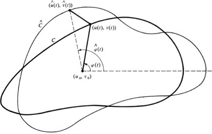
FIGURE 26.7Illustration of Rouch's theorem
For any τ, a ≤ τ ≤ θ, define
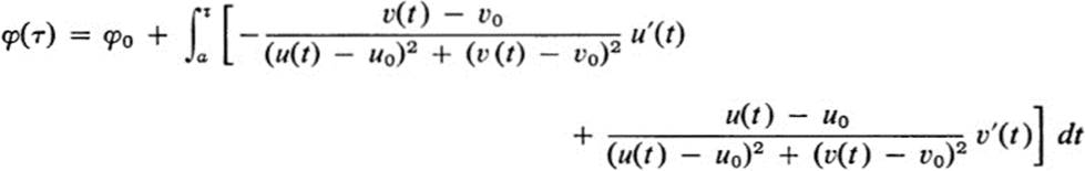
and ![]() similarly. The integrand is d/dt tan-1 [(υ(t) − υ0)/(u(t) − u0)], and these integrals simply define in a continuous way the angles φ(t) and
similarly. The integrand is d/dt tan-1 [(υ(t) − υ0)/(u(t) − u0)], and these integrals simply define in a continuous way the angles φ(t) and ![]() along the curve (see Fig. 26.7). Furthermore,
along the curve (see Fig. 26.7). Furthermore,
![]()
Thus
![]()
where k = n(C; u0,υ0) − n(![]() ;u0, υ0). If k ≠ 0, then the function τ(t) −
;u0, υ0). If k ≠ 0, then the function τ(t) − ![]() increases or decreases by at least 2π as t goes from a to b, and since it is a continuous function, it must be equal to an odd multiple of π for some t0 between a and b. This means that the points (u(t0), υ(t0)) and
increases or decreases by at least 2π as t goes from a to b, and since it is a continuous function, it must be equal to an odd multiple of π for some t0 between a and b. This means that the points (u(t0), υ(t0)) and ![]() lie on a line through (u0, υ0) and on opposite sides of (u0, υ0). But then the distance between these points is greater than the distance from (u(t0), υ(t0)) to (u0, υ0), contrary to assumption. Thus k must equal zero, which is the desired result.)
lie on a line through (u0, υ0) and on opposite sides of (u0, υ0). But then the distance between these points is greater than the distance from (u(t0), υ(t0)) to (u0, υ0), contrary to assumption. Thus k must equal zero, which is the desired result.)
Remark One way to visualize Rouche’s theorem is the following. Let the point (u0, υ0) be the position of the sun, and let C and ![]() be the paths of the earth and the moon, respectively. If after a certain number of orbits the earth and the moon both return to their original position, then C and
be the paths of the earth and the moon, respectively. If after a certain number of orbits the earth and the moon both return to their original position, then C and ![]() will be closed curves. The fact that the distance from the moon to the earth is always less than the distance from the earth to the sun implies that the number of times the moon has gone around the sun must equal the number of times the earth has gone around the sun.
will be closed curves. The fact that the distance from the moon to the earth is always less than the distance from the earth to the sun implies that the number of times the moon has gone around the sun must equal the number of times the earth has gone around the sun.
*26.27 Let G be a differentiable transformation, let G(x0, y0) = (u0,υ0), and suppose that the Jacobian of G at (u0, y0) is different from zero. Let C be the circle x = x0 + rcos t, y = y0 + r sint, 0 ≤ t ≤ 2π and let ![]() be its image under G. Show that for all sufficiently small values of r,
be its image under G. Show that for all sufficiently small values of r,
(Hint: if we set (u, υ) = G(x, y), then by Th. 16.2,
![]()
where ![]() h(x, y)
h(x, y)![]() is a remainder term satisfying
is a remainder term satisfying

Let ![]() be the ellipse that is the image of C under the transformation
be the ellipse that is the image of C under the transformation
Since the determinant Δ of this transformation is
which is assumed nonzero, we may apply Ex. 26.25 and deduce that n(![]() ; u0, υ0) = ± 1 according as Δ > 0 or Δ < 0. If λ2 is the minimum of
; u0, υ0) = ± 1 according as Δ > 0 or Δ < 0. If λ2 is the minimum of
![]()
then the fact that dG(x0,y0) is nonsingular implies that λ2 > 0. Then
![]()
for all (x, y). But for d(x, y) sufficiently small we have |![]() h(x, y)
h(x, y)![]() | < (λ2)1/2 d(x, y). This means that the inequality
| < (λ2)1/2 d(x, y). This means that the inequality

must hold at every point of the circle C for r sufficiently small. But this inequality is precisely the condition on the curves ![]() and
and ![]() which by Ex. 26.26 guarantees that n(
which by Ex. 26.26 guarantees that n(![]() ; (u;0, υ0) = n(
; (u;0, υ0) = n(![]() ;u0 υ0). (Note that the ellipse
;u0 υ0). (Note that the ellipse ![]() of this exercise plays the role of the curve C in Ex. 26.26.)
of this exercise plays the role of the curve C in Ex. 26.26.)
26.28 Let G be a differentiable transformation, let (u0,υ0) = G(x0, y0), and suppose that the Jacobian of G at (x0, y0) is different from zero. Then the image under G of any disk (x − x0)2+(y−y0+ < r2 includes all points in some disk (u − u0)2 + (υ − υ0)2 < R2.(Hint: in the notation of Ex. 26.27, if r is sufficiently small, then the image ![]() of the circle C of radius r about (x0 y0) satisfies n(
of the circle C of radius r about (x0 y0) satisfies n( ![]() u0 υ0) ≠ 0. Choose R so that the disk (u − u0)2 + (υ − υ0)2 < R2 does not contain any points of
u0 υ0) ≠ 0. Choose R so that the disk (u − u0)2 + (υ − υ0)2 < R2 does not contain any points of ![]() . Let (U, V) be any point of this disk. By Ex. 25.18a, n(
. Let (U, V) be any point of this disk. By Ex. 25.18a, n( ![]() ; U, V) = n(
; U, V) = n( ![]() u0, υ0). By Ex. 26.23 above, it follows that (U, V) is the image under G of some point (x, y) inside C.)
u0, υ0). By Ex. 26.23 above, it follows that (U, V) is the image under G of some point (x, y) inside C.)
*26.29 Prove the inverse mapping theorem (Th. 17.3). Specifically, let G(x, y) be a differentiable mapping defined in a domain D by
where f(x, y), g(x, y) ∈![]() in D. Let (u0, υ0) = G(x0, y0) and suppose
in D. Let (u0, υ0) = G(x0, y0) and suppose
Show that there exists a disk D':(x − x0)2 + (y − y0)2 < r2, such that G maps D' one-to-one onto a domain E', and such that G−1 is a differentiable map of E' onto D'. Proceed in the following steps.
a. Choose r sufficiently small so that
![]()
where (x3, y3) and (x4, y4) are any two points of the disk
![]()
Show that G maps D' one-to-one onto a domain E'. (Hint: by Ex. 17.17, it is always possible to choose r so that the given condition is satisfied, and for any such r, the map G is one-to-one in D'. Note that this condition implies in particular that ∂(u, υ)/∂(x, y) ≠ 0 throughout D'. It follows from Ex. 26.28 that the image E' of D' includes a disk about each of its points, hence is an open set. Finally the fact that D' is connected and G is continuous implies that E' is connected. Hence E' is a domain.)
b. Show that the inverse map H: E' → D' which exists by part a is continuous in E'. (Hint: given any point (u1,υ1) in E' let (x1, yx) = H(u1, y1). H continuous at (u1, υ1) means that for any ∈ > 0 there exists δ > 0 such that (u− u1)2 + (υ − υ1)2 < δ ⇒ (x − x1)2 + (y − y1)2 < ∈, where (x, y) = H(u, υ). But this is a consequence of Ex. 26.28 applied at the point (x1 y1) with ∈ = r and δ = R, using the fact that (x, y) = H(u, υ) ⇔ (u, υ) = G(x, y).)
c. Show that if the inverse map H is given by
then φ1(u, υ) ∈![]() and ψ(u, υ) ∈
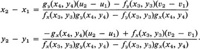
and ψ(u, υ) ∈![]() in E' (Hint: use an analogous reasoning to the proof of the implicit function theorem (Theorem 8.2). Given any two points (u1, υ1), (u2, υ2), in E' let (x1, y1 ), (x2, y2) be the corresponding points in the disk D'. By the mean value theorem applied to the functions f(x, y) and g(x, y), there exist points (x3, y3) and (x4, y4) on the line segment joining (x1, y1 to (x2, y2) such that
in E' (Hint: use an analogous reasoning to the proof of the implicit function theorem (Theorem 8.2). Given any two points (u1, υ1), (u2, υ2), in E' let (x1, y1 ), (x2, y2) be the corresponding points in the disk D'. By the mean value theorem applied to the functions f(x, y) and g(x, y), there exist points (x3, y3) and (x4, y4) on the line segment joining (x1, y1 to (x2, y2) such that
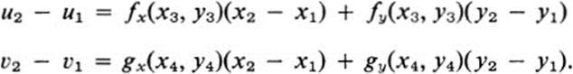
By the condition of part a, these equations can be solved in the form
In order to show the existence of φu(u1, υ1) we choose υ2 = υ1 r and we obtain from the first of the above equations that
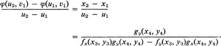
Using the continuity of H (see part b) and the fact that (x3, y3) and (x4, yt) lie on the line between (x1, y1) and (x2, y2) ,we have
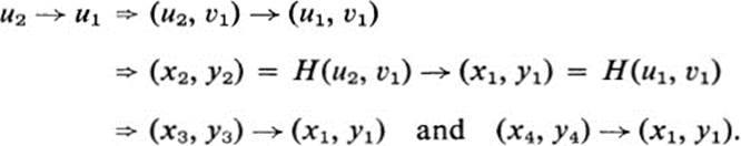
By the continuity of the partial derivatives fx, fy, gx, fx it follows that
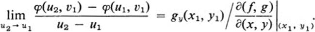
Thus the partial derivative φ(u1, υ1) exists, and in a similar manner, so do φυ, ψu, and ψυ. Furthermore, the expressions for these derivatives show that they depend continuously on x and y, and since x and y are continuous functions of u and υ, the partial derivatives ψu, ψυ, ψu;, ψυ are continuous functions of u and υ.)
*26.30 Let G be a differentiable transformation in a domain D. Let the circle C:x = x0 + r cos t, y = y0 + r sin t, together with its interior, be include in D.Let ![]() be the image of C under G, and let(U, V)be a point not on
be the image of C under G, and let(U, V)be a point not on ![]() . suppose that there are a finite number of points inside C which map onto the point (U,V)and suppose that jacobian of G is not zero at any of these points.
. suppose that there are a finite number of points inside C which map onto the point (U,V)and suppose that jacobian of G is not zero at any of these points.
Specifically, suppose the Jacobian is positive at m points and negative at n points. Then
![]()
(Hint: for each point (xk, yk) inside C such that G(xk, yk) = (U, V), let
![]()
be a small circle, where r is chosen sufficiently small so that all these circles lie inside of C and no two of them intersect. Let ![]() be the image of Ck under G, and let F be the figure consisting of those points which lie on or inside C, and on or outside each Ck. If we define P(u, υ), Q(u, υ) as in Ex. 26.23 and p(x, y), q(x, y) as in Ex. 26.21, then
be the image of Ck under G, and let F be the figure consisting of those points which lie on or inside C, and on or outside each Ck. If we define P(u, υ), Q(u, υ) as in Ex. 26.23 and p(x, y), q(x, y) as in Ex. 26.21, then
But by Ex. 26.27, for r sufficiently small n( ![]() ; U, V) = 1 if ∂(u, υ)/∂(x,y) > 0 at (xk, yk) and n(
; U, V) = 1 if ∂(u, υ)/∂(x,y) > 0 at (xk, yk) and n(![]() ; U, V) = − 1 if ∂(u, υ)/∂(x, y) < 0 at (xk, yk). Thus
; U, V) = − 1 if ∂(u, υ)/∂(x, y) < 0 at (xk, yk). Thus

Remark There are many important special cases of the result in Ex. 26.30. For example, if the mapping G has positive Jacobian everywhere, then the result may be stated as follows: the winding number about a point (U, V) of the image of a circle C is equal to the number of points inside C that map onto (U, V). This is closely related to the so-called argument principle in the theory of functions of a complex variable.
It is most instructive to try to understand the underlying reason for the relation between winding numbers and the number of points that map onto a given point. One way is to picture a disk in the x, y plane made out of a rubber sheet, and to visualize the mapping as a process of distorting this disk by various means, such as stretching, twisting, and folding. When this is done, the resulting form of the rubber sheet may lie in several layers over parts of the u, υ plane, and the number of points in the sheet that lie over a given point corresponds to the number of points inside the original disk that map onto the given point. The study of general properties of mappings such as those considered here belongs to the branch of mathematics known as topology. The specific quantity denoted in Ex. 26.30 by m − n is called the degree of a mapping. For further discussion along these lines we refer to [7], Sections 13-18, and [21], Section 5.