Two-Dimensional Calculus (2011)

Chapter 4. Integration

28. Transformation rule for double integrals

One of the basic methods in the theory of the ordinary integral is that of integration by substitution:

where u is a differentiable function of x for a ≤ x ≤ b, and u(a) = c, u(b) = d. Equation (28.1) describes the behavior of a definite integral when the integrating variable is expressed as a differentiable function of another variable. Our next object is to derive a formula analogous to (28.1) for the double integral.

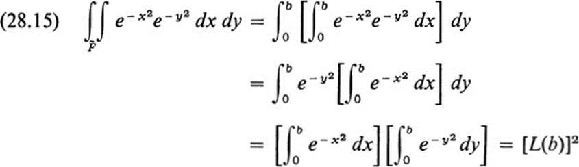
In view of the fact that in the ensuing discussion a single function is expressed in terms of different variables, it is convenient to adopt a modified notation for the double integral. If f(x, y) is integrable over a figure F, we set

The notation on the right is obviously adapted from the iterated integral.

We now state the principal result.

Theorem 28.1 Let F be a figure lying in a domain D of the x, y plane, and let be the image of F under a dijfeomorphism

of D. Let f(u, v) be integrable over . Then

Remark Note the analogy between formulas (28.3) and (28.1). When passing from a differentiable function u(x) to a differentiable transformation u(x, y), v(x, y), it is once again the Jacobian which takes over the role of the derivative. The proofs of (28.1) and (28.3), however, have nothing in common. The proof of (28.1) is a simple application of the chain rule, whereas there is no elementary proof of (28.3). We sketch a proof in the following.⁸

PROOF. Let F₁, …, F_n be an arbitrary partition of F, and let _k be the image of F_k under the transformation G, for k = 1,…, n. Then applying Th. 26.2 and the mean value theorem (Th. 27.1),

where (x_k, y_k) is some point in F_k. Let (u_k, ν_k) be the image of (x_k, y_k) undet the transformation G, denote by the areas of and F_k, respectively. Then multiplying each side of (28.4) by f(u_k, v_k) and adding over k = 1,…, n yields

If we now choose a sequence of partitions whose norm tends to zero, then by the definition of the double integral the right-hand side of (28.5) tends to the integral on the right of (28.3), whereas the left-hand side of (28.5) tends to the integral on the left of (28.3). This proves the theorem.

There are several remarks to be made concerning the above reasoning. First of all, we assumed implicitly that the _k form a partition of , and that the norm of this partition tends to zero with the norm of the corresponding partition of F. Only then can we conclude that the left-side of (28.5) tends to the double integral in (28.3). Furthermore, we have not shown that the integrand on the right of (28.3) is an integrable function. However, in the important case that f(u, v) is continuous on , the function f(u(x, y), v(x, y)). |∂(u, v)/∂(x, y)| is continuous on F, and the integral on the right of (28.3) exists.

Example 28.1

If f(u, v) ≡ 1, then Th. 28.1 reduces to Th. 26.2.

Example 28.2

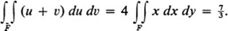
Let be the figure between the lines u + v = 1 and u + v = 2 in the first quadrant. Evaluate ∫∫ (u + v) du dv.

This integral may be evaluated directly, but it is a rather long computation (see Ex. 24.4). Examining the figure , we see that it would be advantageous to introduce the quantity u + v as a new independent variable. We set

Then u + v = 2x, u − v = 2y. Since the figure is given explicitly by

it corresponds under the transformation (28.6) to the figure

or equivalently ( Fig. 28.1),

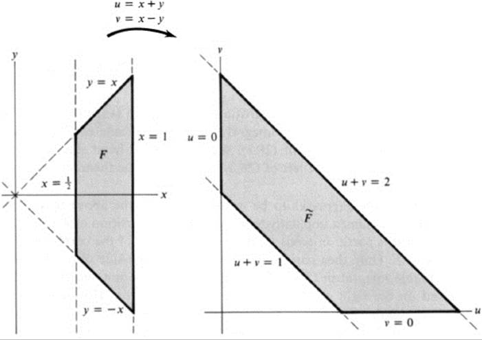
FIGURE 28.1An application of the transformation rule for double integrals

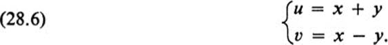
For the transformation (28.6) we have

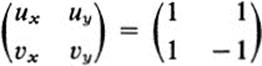
and

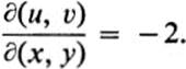
Thus Eq. (28.3) takes the form

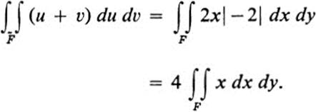
But

and

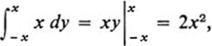
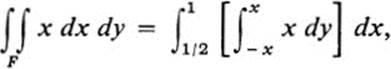
so that

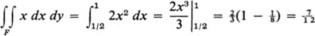
and

There is an important interpretation of Eq. (28.3) that is somewhat different from the version we have presented. Namely, as we have pointed out in the previous chapter, the pair of functions u(x, y), v(x, y) may be considered equally well to define a transformation or a change of coordinates. For example, Eqs. (28.6) amount essentially to a rotation of coordinates, which takes the parallel lines bounding onto a pair of vertical lines bounding F. Another familiar example is

We then have

and

Equation (28.3) takes the form

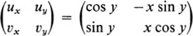
Equations (28.7) may be interpreted as defining a transformation G, or else as introducing new coordinates. Namely, x and y represent polar coordinates in the u, v plane. In the usual notation, setting x = r, y = θ, where it is assumed that r ≥ 0, (28.8) takes the form

Thus, the function f is expressed in polar coordinates, multiplied by r, and then integrated over the corresponding values of r and θ.

Example 28.3

Calculate the y moment of the figure

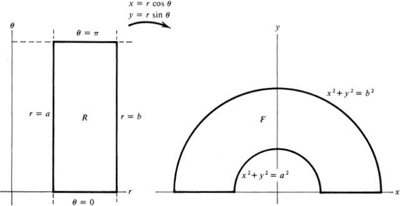
FIGURE 28.2The rectangle in the plane of polar coordinates corresponding to a semi-annulus in rectangular coordinates

If we introduce polar coordinates, the figure F corresponds to the rectangle R:a ≤ r ≤ b, 0 ≤ θ ≤ π ( Fig. 28.2). Thus

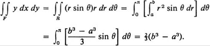
Polar coordinates are certainly, after rectangular coordinates, the most useful and most frequently encountered. In view of this fact, it may be illuminating to give a direct proof of Eq. (28.9), which does not depend on all the theory that was needed to prove the general formula (28.3). We do so for the figure F of Example 28.3 (see Fig. 28.2).

Let f(x, y) be defined on F, and choose a partition of F by figures

where

(see Fig. 28.3). Since the area of a circular sector of angle α is equal to , where r is the radius of the circle, the area of F_ij is equal to

FIGURE 28.3Direct proof of the transformation rule for polor coordinates

Set ρi = (r_i + r_i−1) and choose φ_j, so that θ_j−1 ≤ φ_j ≤ θ_j. Then r_{i −1} < ρi < r_i, and the point whose polar coordinates are (p_i, φ_i) lies in F_ij. Finally, let be the rectangular coordinates of this point. Then

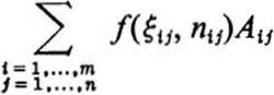
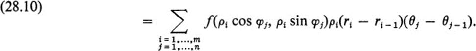
If we take successively finer partitions of F, then the sum on the left-hand side of (28.10) tends to ∫∫_FfdA, by the definition of this integral. On the other hand, if we set

and if we denote by R the rectangle in the r, θ plane defined by a ≤ r ≤ b 0 ≤ θ ≤ π, then the sums on the right of (28.10) are exactly those used in defining the double integral of g over R. Thus, Eq. (28.10) yields in the limit

Remark The essential content of Eq. (28.11) is often written in abbreviated form as

if x and y are rectangular coordinates, and

if r, θ are polar coordinates. Similarly, Eq. (28.3) is abbreviated to

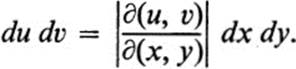
The meaning of these “equations” is that in order to compute the double integral of a function with respect to different sets of coordinates, one need only express the function in terms of the given coordinates, multiply by the corresponding factor, and then evaluate the iterated integral. The term “area element” is often used to denote the expression dA and its representation in various coordinates. It should be understood that these expressions are purely a formalism, just as the corresponding abbreviation du = (du/dx)dx for Eq. (28.1), unless the quantities dx, dy, and their “product” dx dy are suitably defined.

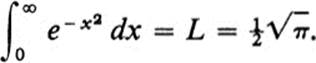
We conclude with an illustration of how some of the ideas introduced in this chapter may be applied to evaluate an important integral. We wish to find the value of

This integral arises in many connections, and plays a special role in the theory of probability. It is a so-called improper integral, since the domain of integration is an infinite, rather than a finite, interval. Its value is defined to be the number

where

Elementary methods of integration do not work, because there is no elementary function whose derivative equals . We observe, however, that we can evaluate the double integral

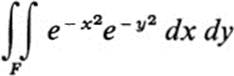
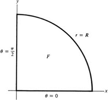
FIGURE 28.4 A quarter disk in polar coordinates

for the figure ( Fig. 28.4)

by introducing polar coordinates.⁹ We have

where is the rectangle 0 ≤ r ≤ R, 0 ≤ θ ≤ θ ≤ π. But

and

On the other hand, if we integrate over the square

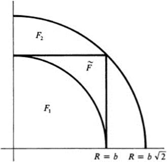
FIGURE 28.5The use of inscribed and circumscribed circles to estimate an integral over a square

we find

using the notation of (28.13). Suppose finally that we consider figures F_l, F₂ of the type F, such that F₁ ⊂ ⊂ F₂ (see Fig. 28.5). For example, for F₁ we set R = b and for F₂ we set R = b . Since the integrand

is positive everywhere, it follows from basic properties of the double integral that

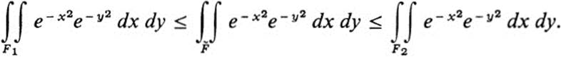
By (28.14) and (28.15), this amounts to

Thus, using the double integral, we obtain specific upper and lower bounds for the value of the ordinary integral (28.13). In fact, the inequalities in (28.16) are remarkably precise because of the rapidity with which the function tends to zero as x tends to infinity. For example, for b = 10, using rough estimates such as

We deduce from (28.16)that

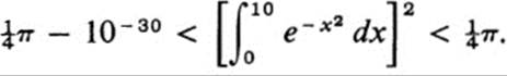
In other words, the square of the integral coincides to the first thirty decimal places with the value π.

To evaluate the original integral (28.12), we let b tend to infinity, and we note from (28.16) that the quantity [L(b)]² is bounded above by π for all b, and is bounded below by a quantity that tends to π as b tends to infinity.

Thus

and

Exercises

28.1Sketch each of the following figures and describe them in terms of polar coordinates.

a. x² + y² ≤ 1, x ≤ 0

b. y ≥0, x ≤ 1, y ≤ x

c. x ≥ 0, y ≥ 0, x + y ≤ 1.

d. −x ≤ y ≤ x, 2ax ≤ x² + y² ≤ 2bx (b > a > 0)

e. a² ≤ x² + y² ≤ 2ay (a > 0)

f. x ≥ 0, (x² + y²)² ≤ a²(x² − y²) (a > 0)

(Note: the figure in part f is bounded by the right-hand loop of the “lemniscate of Bernoulli,” whose equation is (x² + y²)² = a²(x² − y²). Observe that x² − y² ≥ 0 on this figure.)

28.2Compute the area of each figure F in Ex. 28.1 by expressing the integral ∫∫_F 1 dA in polar coordinates and evaluating this integral.

28.3Use polar coordinates to find the centroid of the figures in Ex. 28.1a, b.

28.4Let F be the disk x² + y² ≤ a², a > 0. Express each of the following double integrals as an iterated integral in polar coordinates, and evaluate.

a.

b.

28.5Use polar coordinates to compute the volume of each of the following solids.

a. Under the plane z = c and over the paraboloid z = x² + y², where c > 0.

b. Inside the sphere x². + y² + z² = a², a > 0.

c. Under the surface z = cos (x² + y²),over the disk x² + y² ≤ π in the x, y plane.

d. Under the surface z = cos (x² + y²), and over the annulus, π ≤ x² + y² ≤ 2π.

28.6 Use polar coordinates to compute ∫∫_F Q(x, y) dx dy, where Q(x, y) = ax² + 2bxy + cy² is an arbitrary quadratic form, and F is the disk x² + y² ≤ R².

28.7 Let F be the figure x²/a²+ y²/b² ≤ 1, where a > 0, b > 0. Let be the image of F under the transformation u = x/a, v = y /b.

a. Express ∫∫_F f(x, y) dx dy as an integral over . (Note that the roles of the x, y and u, v planes are reversed here from the way they appear in Eq. (28.3).)

b. Use the formula in part a to evaluate ∫∫_F (x²+ y²) dx dy.

c. Verify that the expression obtained in part a yields the area of F when f(x, y) ≡ 1.

28.8 In each of the following cases there is given a figure F, a transformation G, and a function f(u, v) defined on the image of F under G. Find explicitly and verify Th. 28.1 in each case by evaluating both sides of Eq. (28.3). (Use polar coordinates wherever convenient.)

a.

b. F:x² + y² ≤ 1; G: u= x − y, v = x + y; f(u, v) = u² + v²

c.

d.

28.9 Let be the figure 0 ≤ u + v ≤ 2, 0 ≤ v − u ≤ 2. Evaluate

by applying Th. 28.1 to the transformation G of Ex. 28.8a, and transforming to an integral over the corresponding figure F in the x, y plane.

*28.10Let F be the triangle x ≥ 0, y ≥ 0, x + y ≤ 2. Evaluate

by making a suitable transformation. (Note that the integrand is not defined at the origin, and in fact it cannot be extended in a continuous manner to the origin. However, if we assign an arbitrary value to the function at the origin, the integral exists and is independent of the particular value chosen.)

28.11 Let be the parallelogram with vertices (0, 0), (2, 1), (1, 3), (3, 4). Let G be a linear transformation that maps the square F: 0 ≤ x ≤ 1, 0 ≤ y ≤ 1 onto .

a. Find G explicitly. (Hint: write down a general linear transformation, and find the coefficients by setting G(1,0) = (2, 1), G(0, 1) = (1,3). Then automatically G(1, 1) = (3, 4).)

b. Evaluate ∫∫ (u + v) du dv by expressing this integral as an integral over F.

8.12Given R > 0, let F be the figure 4x² + 9y² ≤ R². Use a suitable transformation to evaluate

28.13Let Q(x, y) = Ax² + 2Bxy + Cy² be an arbitrary positive definite quadratic form.

a. Show that if u = ax + by, v = cx + dy is a linear transformation such that u² + v² = Q(x, y), then the determinant Δ = ad − be satisfies Δ² = AC − B².(Hint: express A, B, C explicitly in terms of a, b, c, d and compute AC − B².)

b. Show that, given the quadratic form Q(x, y), it is always possible to find explicitly a nonsingular linear transformation of the type specified in part a. (Hint: show that the equations expressing A, B, and C in terms of a, b, c, d, can be solved for a, b, c, d in terms of A, B, C. Note that there is quite a bit of freedom in solving; for example, one may choose c = 0, and solve for a, b, d.)

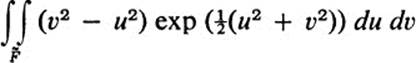
c. Let F be the figure Q(x, y) ≤ R². Evaluate yf∫_F Q(x, y) dx dy.

d. Let F be as in part c. Evaluate

28.14Suppose, under the hypotheses of Th. 28.1, that the function f(u, v) can be written in the form f = h_u, for some function h(u, v) ∈ . Show that Th. 28.1 then follows by the same reasoning that was used to prove Th. 26.2; namely, express ∫∫ h_u(u, v) du dv as a line integral over ∂ , transform this into a line integral over ∂ F, and apply Green’s theorem to obtain an integral over F. (See Ex. 26.22. Note that this reasoning can only work for f(u, v) continuous, and even then the existence of a function h(u, v) satisfying h_u = f is not clear, as we have seen in Ex. 22.18.)

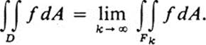
RemarkIt is possible to define improper double integrals in a manner analogous to improper integrals for functions of a single variable. Suppose, for example, that the domain D is the entire x, y plane. A sequence of figures F_k is said to exhaust D if each figure lies in the succeeding one, and if an arbitrarily large disk x² + y² ≤ R² lies in some F_k for sufficiently large k. (An example would be if each F_k were chosen to be the disk x² + y² ≤ k².) The integral of f(x, y) over D is said to converge if

1. ∫∫_F fdA exists for every figure F in D.

2.If these three conditions hold exists whenever F_k exhausts D.

3.The limit in condition 2 is independent of the sequence F_k.

If these three conditions hold, then the (improper) integral of f over D is defined by

Exercises 28.15-28.18 deal with improper double integrals.

*28.15 Suppose that D is the whole plane, f(x, y) ≥ 0 in D, and ∫∫_F fdA exists for every figure F in D. Show that if for some sequence of figures F_k that exhaust D, exists, then for any other sequence of figures _k that exhaust D, exists also, and the two limits are equal. (Hint: since F_k ⊂ F_{k + 1} for each k, and f ≥ 0, it follows that a_{k + 1} ≥ a_k, where a_k = Similarly, if then b_{k + 1} ≥ b_k. Furthermore, each F_k is bounded, hence lies in some disk x² + y² ≤ R², and since the sequence _k exhausts D, this disk lies in _m for some m. Hence for each k there exists an m such that a_k ≤ b_m. Similarly, for each m there exists an n such that b_m < a_n. Deduce that if the (increasing) sequence a_k tends to a limit l, then the (increasing) sequence b_k tends to the same limit.)

Note: if f(x, y) is continuous in D, then condition 1 in the definition of the improper integral certainly holds. If, in addition,f(x, y) ≥ 0, then by Ex. 28.15, condition 3 holds, and it is sufficient to verify that the limit in 2 holds for some sequence F_k. This limit is then the value of the improper integral. Use this fact in Exs. 28.16 and 28.17.

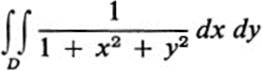
28.16Let D be the entire x, y plane. Evaluate the following expressions.

a.

(Hint: use circular disks for the F_k.)

b.

(Hint: same method as part a.)

c.

(Hint: see Ex. 28.12, and use a suitable sequence of ellipses for the F_k.)

d.

where A > 0, AC — B² > 0. (Hint: see Ex. 28.13, and use a suitable sequence of ellipses for the F_k.)

e.

where A > 0, AC — B² > 0.(Hint: use the same method as part d.)

f.

(Hint: factor the denominator and use a sequence of squares for the F_k.)

28.17Show that if f(x, y) is continuous in the whole plane D, and if 0 ≤ f(r cos θ, r sin θ) ≤ 1/r³, then ∫∫_D f dA converges.

28.18Show that if D is the whole plane, then

does not converge.

28.19The gamma function is defined as an improper integral:

Specifically, if for any positive numbers a, b, we set then Γ(x) = lim_{a →0,b →∞} L(a, b). This limit exists for all x > 0. The function of x so defined is Euler’s answer to the problem of finding a continuous function of x with the property that Γ(n + 1) = n! for each positive integer n.

a. Show that Γ(x + 1) = xΓ(x) for each x > 0. (Hint: integrate by parts, differentiating e^−t and integrating t^{x− 1} (x being fixed); take the limit as a → 0 and b → ∞.)

b. Show that Γ(1) = 1.

c. Deduce from parts a and b that Γ(n + 1) = n! for positive integers n.

d. Show that Γ( ) = (Hint: make the substitution t = u² in the definition of Γ( ), and use the value found for the integral (28.12).)

¹ Actually the statement in Lemma 21.1 is more general than what is usually referred to as “change of parameter,” since we do not assume that the function h(τ) is monotone; that is, that the correspondence between τ and t is one-to-one

² For further discussion and a proof of the fundamental theorem, see [14], Sections 3.4, 3.5, and 9.5.

³ The development followed here is in broad outline an adaptation to two dimensions of the treatment of multiple integration given by Maak [25]. Some changes in approach and organization make it impossible to give specific references in Maak’s book for results stated here without proof. However, with the exception of one point in the proof of Th. 23.3 (see Footnote 6, p. 335) all results stated in this and the following section are consequences of the theorems proved (in the n-dimensional case) in the first three sections of Chapter 11 of Maak. For a different treatment of multiple integration, carried out specifically in the case of two dimensions, see [6], Sections 3.1 and 3.2.

⁴ The procedure described in the definition of area may be applied to any bounded set of points F. Even if F is not a figure, the numbers A_k will still converge to a number A which is called the inner area of F. However, for complicated point sets F, the inner area so defined will not have the basic properties listed in Th. 23.1.

⁵ The proof for a general figure follows from Th. 17 in Chapter III of [16]. The function f in that theorem should be chosen to be equal to 1 at each point of F, and equal to 0 everywhere else.

⁶ The fact that the integral (23.7) exists follows in the general case from the reference given in the previous footnote. In the special case of polynomial figures one can show that the function h(t) is bounded and continuous except for at most a finite number of values of t, from which the existence of the integral (23.7) follows immediately.

⁷ For a different method of proof, which applies to an arbitrary figure, see [28], Sections 14.1–14.3.

⁸ For a complete proof, as well as an interesting discussion of the advantages and disadvantages of each of the standard proofs, see [32]. See also Ex. 28.14, at the end of this section.

⁹ Strictly speaking, Th. 28.1 does not apply in this case since the figure F contains the origin, and the transformation x = r cos π, y = r sin π is not a diffeomorphism in any domain containing a point where r = 0. However, it is easy to show that the conclusion of Th. 28.1 still holds in this case, either by excluding a small circle of radius ∈ about the origin and taking the limit as ∈ tends to zero, or else by using the special reasoning for polar coordinates, which led to Eq. (28.11)