Two-Dimensional Calculus (2011)

Chapter 2. Differentiation

4. Partial derivatives and plane domains

The first observation to be made in the study of a function of two variables f(x, y) is that when either x or y is held fixed the function is reduced to one of a single variable. The ordinary derivative with respect to that variable is called a partial derivative of the original function. To be precise we make the following definition.

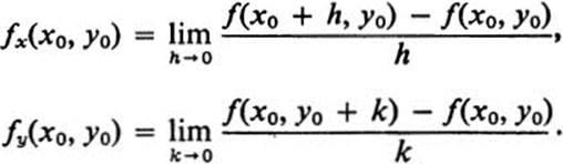
Definition 4.1 The partial derivative of f(x, y) with respect to x at the point (x₀, y₀) is denoted by f_x(x₀, y₀) and is defined by

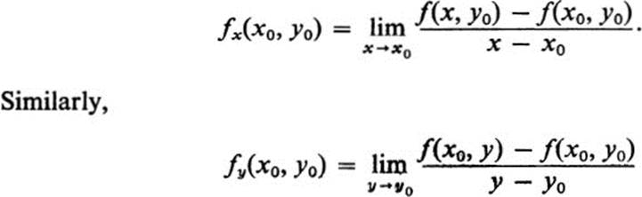
is called the partial derivative of f(x, y) with respect to y at the point (x₀, y₀).

There are many different notations currently used for partial derivatives. Among the most common are

In this book we will generally use f_x and f_y, but occasionally also ∂f/∂x, ∂f/∂y. Also, when we set z = f(x, y), we write z_x, z_y and ∂z/∂x, ∂z/∂y.

Returning to the definition, we see that in each case we have kept one of the variables fixed and formed the ordinary derivative with respect to the other variable. It follows immediately that all the basic laws concerning ordinary derivatives give rise to corresponding laws for partial derivatives. These include the rules for differentiating sums, products, and quotients. In particular, if ∂f/∂x and ∂g/∂x both exist at (x₀, y₀), then so do ∂(fg)/∂x and, providing g(x₀, y₀) ≠ 0, ∂(f/g)/∂x. Similarly for the partial derivative with respect to y. As a result, if f is a polynomial, then f_x and f_y exist at every point.

Example 4.1

If

then

Note that to take the partial derivative with respect to one variable we simply treat the other variable as a constant.

Example 4.2

If

then

Example 4.3

If

then

Note that here we have to use the chain rule. We have

To take the partial derivative with respect to x, we consider y constant, and we multiply the derivative of f with respect to u by the derivative of u with respect to x.

Example 4.4

If

then

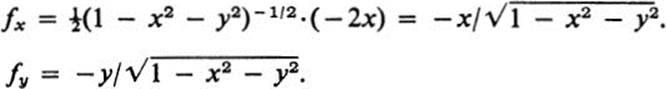
This last example is very instructive. Note that the function f is defined for x² + y² ≤ 1. The functions f_x and f_y are well-defined at all points inside this circle, that is, for x² + y² < 1. However, when x² + y² = 1, although f is defined, the expressions for f_x and f_y have a zero in the denominator. If we recall the definition of partial derivatives, we see that they are actually not defined at points (x₀, y₀) where ; indeed, the expression whose limit we wish to take is not defined for all x sufficiently near x₀. It would be possible to consider one-sided limits and derivatives, but at certain points even these are not defined. For example, f(x, 1) is defined only for the single value x = 0 (Fig. 4.1), and f_x(0, 1) does not exist in any sense.

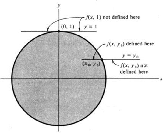
FIGURE 4.1 The domain of definition of

Thus, before we proceed to compute partial derivatives blindly and obtain meaningless results, we should look a little more closely at the domain of definition of a function. In particular, we have to distinguish between those interior points where we may apply any differentiation rule from singlevariable calculus without hesitation and the boundary points where trouble may arise.

We are confronted here with the first essential distinction between functions of one variable and functions of two variables. A function of one variable is defined on an interval or a set of intervals. A function of two variables may be defined on a very complicated domain in the plane. Even relatively simple functions, such as f(x, y) = (P(x, y))^1/2, where P is a polynomial, may lead to quite complicated geometrical figures. More generally, the function

where P₁, ..., P_n are polynomials, is defined on the set of points satisfying all of the inequalities

We have already seen examples of such functions, including the one we have just discussed, where P(x, y) = 1 – x² – y². The following are some typical examples.

Example 4.5

For this function to be defined, we must have

which describes a domain bounded by an ellipse (Fig. 4.2).

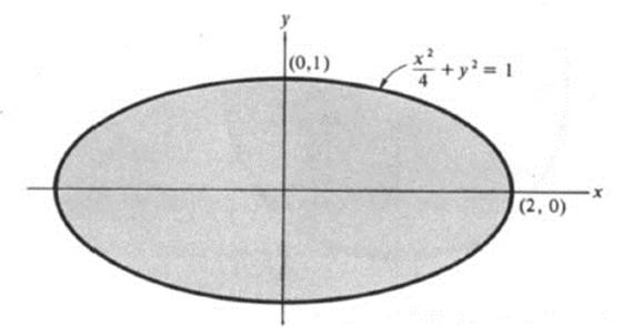
FIGURE 4.2 The set of points satisfying (x²/4) + y² ≤ 1

Example 4.6

This function is defined, except when the two factors under the radical have opposite sign. Thus the function is defined only for those points (x, y) satisfying both

or both

The Eqs. (4.4) cannot be simultaneously satisfied, since they assert that x² + y² is a number at most equal to 1 and at least equal to 4. Thus the function is defined only for the set of points satisfying Eqs. (4.3); that is, the set of points bounded by the circles of radius 1 and 2 about the origin (Fig. 4.3). A set of points of this type (bounded by two concentric circles) is called an annulus.

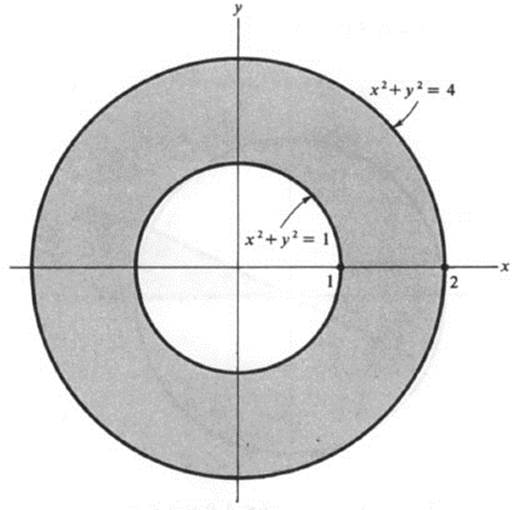
FIGURE 4.3 The annulus 1 ≤ x² + y² ≤ 4

Example 4.7

Here y ≥ x² and y ≤ 1, which is a parabolic segment (Fig. 4.4).

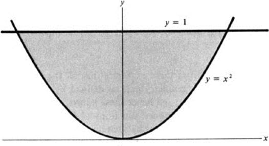
FIGURE 4.4 The parabolic segment x² ≤ y ≤ 1

Example 4.8

We have

This defines a circular sector (Fig. 4.5).

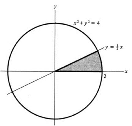
FIGURE 4.5 The circular sector x² + y² ≤ 4, 0 ≤ y ≤ x/2

Example 4.9

This function is defined in the rectangle (Fig. 4.6):

Example 4.10

See Fig. 4.7.

It is probably clear from these examples that all the figures one usually encounters in elementary geometry can be defined by a set of polynomial inequalities of the form (4.2), and hence these figures are the precise domains of definition of certain elementary functions (4.1). Clearly, one can also obtain far more complicated figures by such inequalities. For our purposes it makes little difference how simple or complicated a figure may be. The

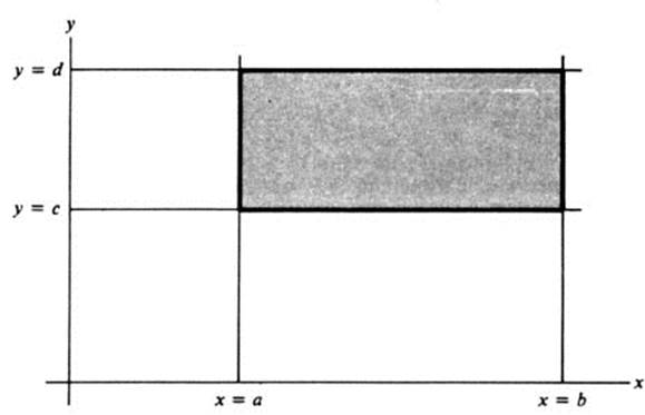
FIGURE 4.6 The rectangle a ≤ x ≤ b,c ≤ y ≤ d

important thing is to distinguish between its interior points and boundary points. We do this as follows.

Definition 4.2 Let S be any set of points in the plane. A point (x₀, y₀) is called a boundary point of S if

1. There are points of S arbitrarily close to (x₀, y₀);

2. There are points not in S that are arbitrarily close to (x₀, y₀).

A point of S that is not a boundary point is called an interior point of S.

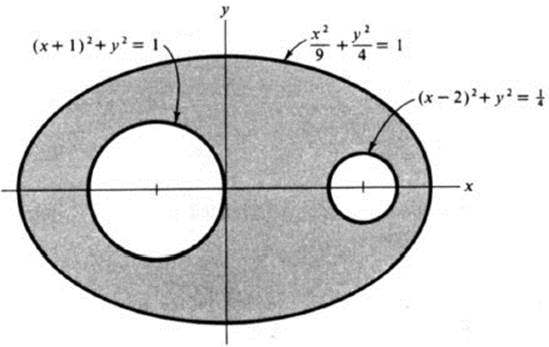
FIGURE 4.7 The set of points satisfying 4x² + 9y² ≤ 36, (x + 1)² + y² ≥ 1 and 4(x − 2)² + 4y² ≥ 1

Remark An interior point of S, by its definition, is always a point of S, whereas a boundary point of S may or may not itself belong to S.

Example 4.11

If S is the set of points satisfying x² + y² ≤ 1, then the points on the circle x² + y² = 1 are the boundary points of S, and those satisfying x² + y < 1 are interior points of S.

Example 4.12

If S is the set of points satisfying x² + y² < 1, then again all points on x² + y² = 1 are boundary points of S, while all points x² + y² < 1 are interior points.

Note that in Example 4.12, every point of S is an interior point. As we mentioned earlier, we want to restrict our attention to sets having this property as the domains of definition of our functions, in order to be able to differentiate freely.

Definition 4.3 A set S of points is called open if every point of S is an interior point.

Examples of open sets are those sets of points (x, y) which satisfy a set of strict inequalities

where P₁, P₂, ..., P_n are polynomials. In fact, nothing is lost in this or the next chapter if functions are pictured as being defined on such sets. There is, however, one further restriction that is convenient to make. An open set may consist of several disconnected parts, and it is sufficient to study the function separately on each part. For example, the set consisting of those points (x, y) satisfying both

consists of the two shaded domains indicated in Fig. 4.8, lying inside an ellipse and outside a circle.

Definition 4.4 An open set S is connected if for any two points of S there is a curve lying in S joining the two points.

Definition 4.5 A domain is a connected open set.

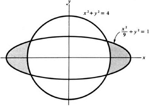
FIGURE 4.8 The set of points satisfying (x²/9) + y² < 1, x² + y² > 4

We adhere to this terminology throughout the book. Whenever we speak of a function defined in a domain D, we mean that D is a set of points of this specific nature.

Remark The expression “the domain of a function” is often used to mean the set of points on which a function is defined. This set of points may or may not be “a domain” in our sense. In the following, we always refer to “a function defined in a domain D,” with the understanding that the function may be defined at other points too, but that we are restricting our attention to the behavior of the function in D.

Example 4.13

Let D be the set of points (x, y) such that x² + y² < 1. The following functions are defined in D:

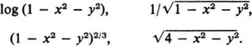
The first two of these functions are defined precisely at points of D and nowhere else. The third is also defined at boundary points of D, but as we have seen, its partial derivatives are not. The last is actually defined in a larger domain, but we may wish to consider only the values that it takes on in D.

A basic ingredient of the above definitions is the notion of “all points sufficiently close to a given one.” This notion can be formalized as follows.

Definition 4.6 A neighborhood of a point (x₀, y₀) is the set of all points (x, y) lying in some disk (x – x₀)² + (y − y₀)² < r².

This terminology leads to a convenient characterization of interior points and boundary points. Given a set S and a point (x₀, y₀), (x₀, y₀) is an interior point of S if and only if some neighborhood of (x₀, y₀) lies entirely in S, and (x₀, y₀) is a boundary point of S if and only if every neighborhood of (x₀, y₀) contains at least one point of S and one point not in S (see Ex. 4.16 and Fig. 4.9).

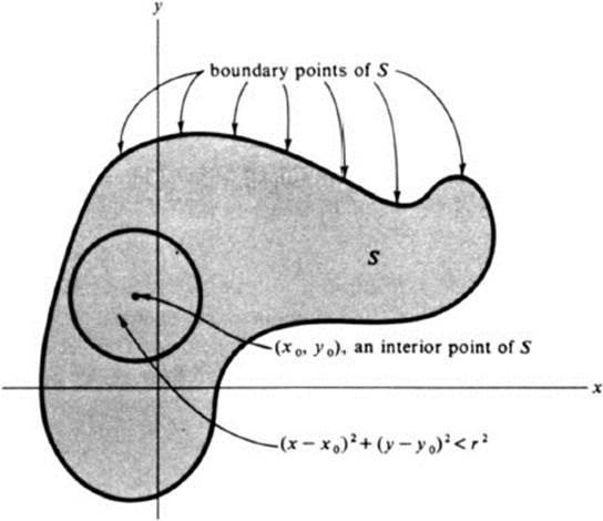
FIGURE 4.9 Boundary points and interior points

Exercises

4.1 Find the partial derivatives with respect to x and y of each of the following functions f(x, y).

a. x⁴ + 3x²y − 5xy³

b. x² + 2xy + y²

c. x³ + 3x²y + 3xy² + y³

d. (x + y)⁵

e. sin (x + y)

f. sin (x² + y²)

g.

h. (x³ + y³)^1/3

i. arc tan (y/x)

j. xe^y/x

k. xy/(x² + y²)

l. xy sin xy

m. sec³ x log x + 5

n. log tan (x + y²)

4.2 Find the value of the following partial derivatives at the points indicated.

a. f_x(0, 0) if f(x, y) = sin (xe_y)

b. f_y( π, 0) if f(x, y) = log (sin x + sin y)

c. f_x( π, 1) if f(x, y) = e^{y tan x}

d. f_y(0, 0) if f(x, y) = cosh x sin y

4.3 Compute the expression xf_x + yf_y for each of the following functions f(x, y).

a. x³ + y³

b. (x + y)³

c.

d.

4.4 Compute the partial derivatives of the following pairs of functions, and show that they satisfy the equations f_x = g_y, f_y = −g_x.

a. f(x, y) = e^x cos y, g(x, y) = e^x sin y

b.

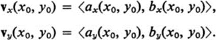
4.5 If a(x, y), b(x, y) are given functions, and if for each point (x, y) we consider the vector

then the partial derivatives of v(x, y) are defined by

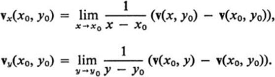
Show that

4.6 Let v = ⟨a, b⟩, w = ⟨c, d⟩ be vectors, where a, b, c, and d are all functions of x and y. Suppose that λ is also a function of x and y. Show that

a.

b.

c.

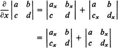
4.7 Using the notation

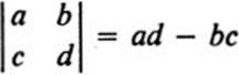
for a 2 × 2 determinant, show that if a, b, c, d are functions of x and y, then

*4.8 State and prove a corresponding result for a 3 × 3 determinant.

4.9 Compute the determinant for the following pairs of functions

a. f(x, y) = x² − y², g(x, y) = 2xy

b. f(x, y) = e^x cos y, g(x, y) = e^x sin y

c. f(x, y) = x² + y² + 2xy + 2, g(x, y) = e^xe^y

d. f(x, y) = x − 2 log y, g(x, y) =

4.10 Let f(x, y) = sin xy.

a. Show that xf_x − yf_y ≡ 0.

b. Let F(t) be an arbitrary differentiable function of one variable, and let g(x, y) = F(f(x, y)). Show that also xg_x − yg_y ≡ 0.

4.11 Show that Def. 4.1 that we have given for partial derivatives is equivalent to the following:

4.12 By referring directly to the definition of partial derivatives, compute f_x(0, 0) and f_y(0, 0), where

a. f(x, y) = x − y²

b. f(x, y) = 1 + x cos y

*c.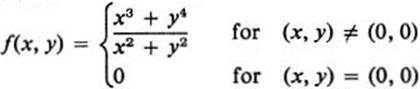

*d.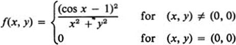

4.13 Find the set of points where each of the following functions is defined, and sketch.

a.

b.

c. log x + 1/ + (1 − x − y)^−1/4

d. arc sin x + arc cos y

4.14 Describe the boundary points of each of the following sets of points (x, y). Illustrate with a sketch.

a. x² + 4y² < 4

b. x² + 4y² > 4

c. x² + 4y² ≥ 4 and x² + 4y² ≤ 16

d. x ≥ 2y and y ≥ 2x

e. x² ≤ 1 and y² ≤ 4

f. x² + y² = 1

4.15 a. Which of the sets in Ex. 4.14 are open?

b. For each set in Ex. 4.14 which is not open, name a point of the set that is not an interior point.

4.16 Show that the following characterizations of boundary points and interior points of a set S are equivalent to the definitions in the text. A point (x₀, y₀) is a boundary point of S if for every positive number r, the disk (x − x₀)² + (y − y₀)² < r² contains at least one point in S and at least one point not in S. A point (x₀, y₀) is an interior point of S if for some positive r (sufficiently small), all points of the disk (x − x₀)² + (y − y₀)² < r² are in S (Fig. 4.9).

4.17 A set S is called closed if S contains all its boundary points. Which sets in Ex. 4.14 are closed? (Note that a set S may be neither open nor closed. This happens when S contains some of its boundary points, but not others.)

4.18 A set S is called convex if for any two points of S, all points on the line segment joining them also lie in S.

a. Which sets in Ex. 4.14 are convex? (Do not try to justify your answers. This is one place where geometric intuition is almost infallible. Actual proofs are not difficult, but they require some practice in juggling inequalities.)

b. Show that an open convex set is necessarily a domain.

4.19 Prove carefully, by referring directly to the definition, that each of the following sets is a domain

a. the whole plane

b. the half-plane y > 0

c. the disk x² + y² < 1

4.20 Show that for the following functions f(x, y) the partial derivatives do not exist at the points indicated

a.

b. f(x, y) = (x + y − 3)^1/3 at (1,2)

(Note that both functions are defined throughout the plane.)