Homework Helpers: Physics
1 Kinematics
Lesson 1–6: Graphing Motion
Graphs are important tools for physics. If you can interpret graphs correctly, you will be able to extract a great deal of information from them quite quickly. Being able to construct graphs properly will give you the ability to summarize results in a format that is easy to read. This lesson will focus on the interpretation of motion graphs.
The first type of graph that we will study is called a position vs. time graph. Perhaps the quickest way to learn how to interpret this type of graph is to construct one. Let”s go back to studying the motion of our friendly squirrel from Lesson 1–1. For the sake of simplicity, let”s imagine that the squirrel is capable of changing its velocity instantaneously, so that it takes it no time to accelerate between two different velocities. For any period of time, the velocity of the squirrel will be uniform, which means that its instantaneous velocity will be the same as its average velocity for that period of time.
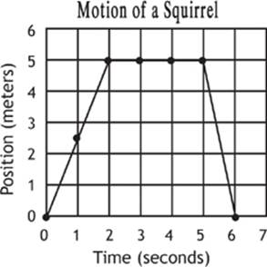
Let”s imagine that when we first observe the squirrel it is at the base of a tree, the origin, or starting point. As we watch it, it moves in a straight line with uniform velocity for 2.0 seconds, at which point it stops at a distance of 5.0 m from the origin. We could graph the motion of the squirrel during this time as shown in Graph 1.1.
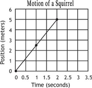
Graph 1.1
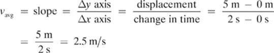
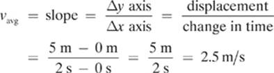
Notice that we can determine the position of the squirrel at any point in time by tracing back to the appropriate axis. For example, at 1.0 second, the squirrel was 2.5 meters away from the tree. We can also determine the average velocity of the squirrel, or the instantaneous velocity for any point if the velocity is uniform, during this period of time by finding the slope of the line! We simply pick two convenient points on the straight line segment, such as (0,0) and (2,5), and put them into the slope formulas, as shown here:
Let”s imagine that the squirrel stops at this point and stays still for a period of 3.0 seconds. Let”s add this data to our graph and see what it looks like (Graph 1.2).
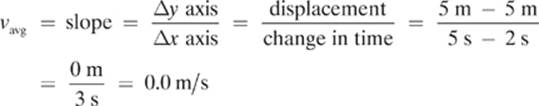
We can see that the line representing the period of time when the squirrel was motionless (from 2.0 s to 5.0 s) is represented by a horizontal line. This makes sense because the slope of this line segment, and therefore the average velocity of the squirrel during this period of time, will be zero, as shown here:
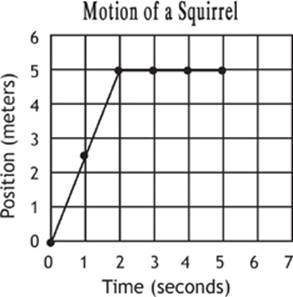
Graph 1.2
Next, let”s imagine that our squirrel is startled by a loud noise, and sprints back to the tree in 1.0 s (this is a really fast squirrel!). Adding this part to our graph would give us the one shown in Graph 1.3.
As the squirrel returns to the tree (origin), the data creates a line segment with a negative slope and, therefore, a negative average velocity as shown here:
Graph 1.3
What does the negative velocity represent? A negative velocity is simply a velocity in the direction that is opposite to the direction that we called positive. The squirrel went back to the tree.
If the squirrel goes past the origin, beyond the tree, this line of his motion will dip below the x-axis, as shown in the next graph. The slope of the line segment would, of course, depend on how fast the squirrel went. For the sake of argument, let”s imagine that the squirrel travels with a velocity of –1.0 m/s during this time (Graph 1.4).
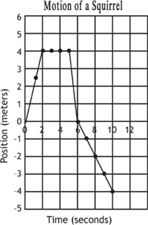
Graph 1.4
Let”s summarize what we have learned about position vs. time graphs.
Position vs. Time Graphs
1. Uniform velocity is represented by a straight line segment.
2. For uniform velocity, the instantaneous velocity is the same as the average velocity.
3. The slope of a line segment shows the average velocity of the object during a period of time.
4. A positive slope represents a positive velocity.
5. A horizontal line with a slope of zero represents a velocity of zero.
6. A negative slope represents a negative velocity.
7. When the line drops below the horizontal axis, the object moves past the origin, heading in the direction designated as negative.
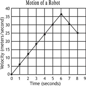
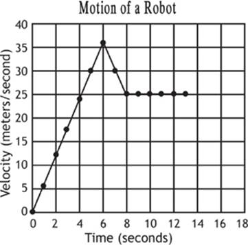
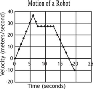
The next type of graph that you will want to be able to create and read is a velocity vs. time graph. For fun, let”s imagine that the students of an advanced physics course have just completed a robot that they have been working on, and they bring it to the gym to test its range of motion. They hit the On button, and the robot goes berserk! A student collects data about the velocity of the robot and wants to summarize the data on a graph, as shown in the following paragraphs.
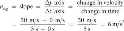
After the robot was turned on, it accelerated at a uniform rate from rest to 36.0 m/s in only 6.0 seconds. This period of the robot”s motion could be graphed as shown in Graph 1.5.
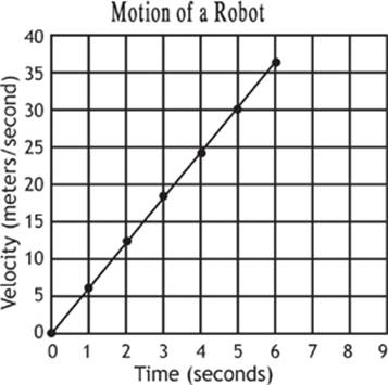
Graph 1.5
Notice that this graph looks very much like our position vs. time graph. We can only tell the difference by paying attention to the label on the y-axis, which is why teachers tend to deduct credit from students who don”t label their graphs properly. The fact that the robot”s motion can be described with a straight line here indicates that the acceleration was uniform.
We can find the velocity of the robot at any time given on the graph, by tracing back to the y-axis. Can you see, for example, that at 5 seconds the robot was traveling with a velocity of 30 m/s?
To calculate the robot”s acceleration during this period of time, we find the slope of the line. I recommend that you choose to compare two points on the line that are very clear. For example, look again at the point on the graph that represents the robot”s velocity at 5 seconds. It seems to fall clearly at 30.0 m/s, so that is a good point to use in our comparison. We can also use the origin, which shows us that the velocity of the robot at 0 seconds was 0 meters/second.
Another interesting thing about these velocity graphs is that we can calculate the displacement of an object by looking at the area under the curve. Look at Graph 1.5 and notice the area under the line and above the x-axis represents a triangle.
If we use the formula for the area of a triangle (![]() base × height), we can find the displacement of the robot during this period of time.
base × height), we can find the displacement of the robot during this period of time.
Given: Base = 6 s Height = 36 m/s
Find: Displacement
![]()
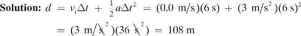
So, the robot travels 108 meters (let”s ignore the fact that this seems to be an unusually large gym!) during the first 6 seconds. If you doubt our answer, you could always check it with one of our formulas for uniform motion. From the graph we can tell that the robot”s initial velocity was 0 m/s, its final velocity was 36 m/s, and the change in time was 6 s. Let”s use this information and the acceleration of 6 m/s2 that we found using the slope formula to solve for displacement.
Given: vi = 0 m/s vf = 36 m/s Δt = 6 s a = 6m/s2
Find: d
Next, let”s suppose that the robot spends the next two seconds slowing down to a velocity of 25.0 m/s. We can add that data to Graph 1.6. (See page 55.)
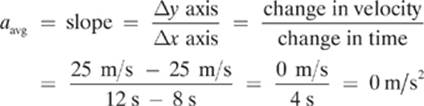
To find the acceleration of the robot from 6 seconds to 8 seconds, we find the slope of the line. The point representing the velocity of the robot at 7 seconds is a little unclear, so let”s compare the velocity of the robot at 6 seconds to the velocity of the robot at 8 seconds.
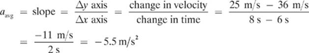
This time we ended up with a negative acceleration. Because the velocity prior to this acceleration was positive, this negative acceleration results in a decrease in velocity. As I mentioned before, a negative acceleration doesn”t always result in a decrease in velocity, but, in this case, it did.
Graph 1.6
Once again, you could find the displacement of the robot during this time by finding the area under the graph. If you wanted to find the displacement of the robot from 6 s to 8 s, you could break the area under that part of the graph into one triangle and one rectangle.
We would find the area of the two shapes and add them together to get the total displacement during this time.
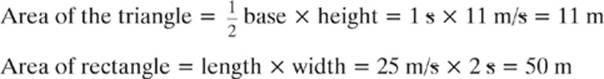
Total displacement = 11 m + 50 m = 61 m
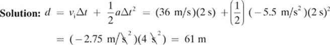
Once again, we could check our method with our equation for uniform motion, as shown here:
Given: vi = 36 m/s vf = 25 m/s Δt = 2 s a = –5.5m/s2
Find: d
Imagine that the robot maintains this velocity for 5 seconds, bringing us to the 13 second mark. Let”s add this information to our graph (Graph 1.7 on page 56).
At a quick glance, you might think that the robot is stationary from 8 seconds to 13 seconds because the slope of the line is zero. However, the robot is still traveling quite fast during this time! It is not the velocity that is zero—it is the acceleration.
It is not the velocity that is zero. Rather, the change in velocity during this period of time is zero. You can tell that the robot is still moving because he is still covering the distance under the curve ![]() during this time.
during this time.
Now the robot experiences a constant acceleration of –5.0 m/s2 for the next 7 seconds. Let”s add this data to our graph (Graph 1.8).
Graph 1.7
Graph 1.8
What has that crazy robot done this time? It changed directions! Can you see what portion of the graph represents a change in direction? The negative acceleration that the robot experienced caused it to slow down from 13 seconds to 18 seconds. At 18 seconds, the velocity of the robot was actually 0 m/s. Once the line dropped below the origin, you can see that the robot has a negative velocity, so it is heading in the opposite direction to what was considered positive. At this point, the robot is actually speeding up in the negative direction.
Let”s summarize what we have learned.
Velocity vs. Time Graphs
1. Uniform acceleration is represented by a straight line segment.
2. For uniform acceleration, the instantaneous acceleration is the same as the average acceleration.
3. The slope of a line segment shows the average acceleration of the object during a period of time.
4. A positive slope represents a positive acceleration.
5. A horizontal line with a slope of zero represents an acceleration of zero.
6. A negative slope represents a negative acceleration.
7. The area under the graph represents the displacement.
8. When the line drops below the horizontal axis, the object changes direction.
Lesson 1–6 Review
1. What does the slope of the line on a position vs. time graph represent?
2. What would a negative velocity look like on a position vs. time graph?
3. What would a uniform acceleration look like in a velocity vs. time graph?