Liquid-State Physical Chemistry: Fundamentals, Modeling, and Applications (2013)

11.5. The Regular Solution Model

Because deviations from the ideal solution behavior occur frequently, an improvement over the ideal solution model is required. These improvements can be classified according to whether they improve upon the enthalpy, the entropy, or both.

The nomenclature used is indicated in Table 11.3. However, it should be borne in mind that other authors frequently deviate from this terminology.

Table 11.3 Nomenclature for solutions.

a) Guggenheim refers to this type as a simple solution.

b) This might also be called a real solution.

In this section we deal with the regular solution model of solute 2 in solvent 1. Hence, we discuss only energetic interactions because in this model the entropy is given by the perfect solution model, Eq. (11.18). With respect to the excess enthalpy there are two options. First, the enthalpy change is positive, that is, H^E > 0 which occurs if the 1–2 interaction is unfavorable. Second, the enthalpy change is negative, that is, H^E < 0 which is the case when the 1–2 interaction is favorable. Our task is thus to model H^E, which equals Δ_mixH because in the perfect solution model Δ_mixH = 0.

We derive the expression for Δ_mixH from the lattice model with coordination number z. As described in Section 11.4, we assume a random distribution of molecules over the lattice, and consider nearest-neighbor interactions only. For a binary system of components 1 and 2 we must then consider the 1–1, 2–2, and 1–2 pair interactions with an interaction w₁₁, w₂₂ and w₁₂, respectively⁶⁾. If we create two 1–2 bonds from a 1–1 and a 2–2 bond, the interchange energy per bond w is given by

(11.54)

where w represents the interchange energy per bond, and zw represents the interchange energy for replacing on molecule 1 (2) by one molecule 2 (1) in the matrix of molecules 1 (2). If N₁ (N₂) denotes the number of type 1 (2) atoms and N = N₁ + N₂ is the total number of atoms, the probability of having an arbitrary site occupied by a molecule of type 1 (2) is x₁ = N₁/N (x₂ = N₂/N). Hence, the probability for a (nearest-neighbor) pair 1–2 is x₁x₂, and similarly for a pair 2–1. The total probability for a pair is thus 2x₁x₂ and consequently, because the total number of pairs is ½zN, the number of 1–2 pairs is ½zN·2x₁x₂ = zNx₁x₂. Similarly, the number of 1–1 pairs is ½ and the number of 2–2 pairs is ½.

The resulting interaction energy of mixing is then

(11.55)

This yields for one mole after a small calculation using N = nN_A

(11.56)

Since for an ideal solution U_m = x₁u₁ + x₂u₂ = ½zw₁₁x₁ + ½zw₂₂x₂, we also have U^E = Δ_mixU. For now, we interpret U as internal energy but come back to this interpretation later. Since in this model volume effects are absent (and in practice are often small), we thus also have for the enthalpy

(11.57)

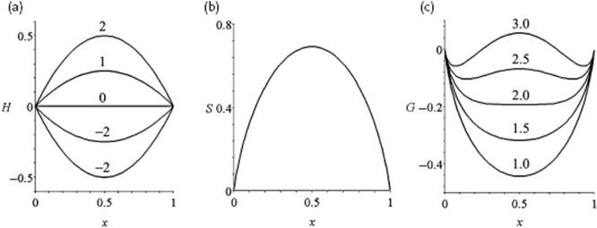
Figure 11.4 shows the behavior of Δ_mixH_m for various values of the parameter zw.

Figure 11.4 (a) The enthalpy of mixing H = Δ_mixH/RT; (b) The entropy of mixing S = Δ_mixS/R; (c) The Gibbs energy of mixing G = Δ_mixG/RT for various values of the interaction parameter zw, all as a function of mole fraction x.

The excess Gibbs function G^E = ΔG − ΔG^ideal can now easily be calculated. For ideal solutions, we calculated the Gibbs energy from the ideal mixing entropy only, as the enthalpy change was considered to be zero. In the case of regular solutions we still use the ideal mixing entropy Eq. (11.18) (also plotted in Figure 11.4), in spite of the preferential interactions, and reading

(11.58)

Hence, we also have G^E = H^E = Nzwx₁x₂. Finally, the molar Gibbs energy of mixing is given by

(11.59)

In Figure 11.4 the behavior of Δ_mixG_m is sketched for various values of the parameter zw. We see that, depending on the value of the parameter zw, Δ_mixG_m shows a single or a double minimum; the latter situation leads to phase separation, to be discussed later.

Problem 11.9

Show that for the regular solution model volume changes are absent as long as the parameter zw is assumed to be pressure-independent.

11.5.1 The Activity Coefficient

The next step is to calculate the activity coefficients. To that purpose we recall that

(11.60)

The chemical potential⁷⁾ is given by , so that G becomes

(11.61)

Since the Gibbs energy for the ideal solution is given by

(11.62)

we thus have

(11.63)

The activity coefficient γ_α (convention I) thus can be calculated from

(11.64)

In the previous paragraph we derived using the regular solution model for the excess Gibbs energy

(11.65)

Hence, the result for the activity coefficients, with β = 1/kT, is

(11.66)

11.5.2 Phase Separation and Vapor Pressure

Mixtures are not always solutions, and from the above model we can assess the phase behavior of a mixture. The critical point for phase separation can be obtained from

(11.67)

Because μ = μ° + RT lna = μ° + RT lnγ x and and , we have

(11.68)

(11.69)

These equations are satisfied for x₁ = x₂ = 0.5 (as would be expected on symmetry grounds) and (βzw)_cri = 2. The critical temperature T_cri for phase separation is thus

(11.70)

At this point the activity coefficient is ln γ = 0.5 or γ = 1.649, and the activity becomes a = γ x = 0.824. In fact, using the expression for Δ_mixG, we can obtain the complete solution of the phase separation problem via ∂Δ_mixG/∂x₂ = 0. This leads to

(11.71)

Using the transformation s = 2x₂ − 1 the final solution is

(11.72)

representing the familiar implicit, zeroth order (or mean field) solution in x₂ for the order–disorder problem (see Appendix C).

The total pressure in the regular solution model becomes

(11.73)

and at T_cri becomes

(11.74)

to be compared with for completely insoluble liquids and for completely soluble liquids. To check the agreement with experiment we use the experimental vapor pressure P_exp for equimolar solutions. From Eq. (11.73) we obtain . It appears that normally the value of zw decreases with increasing temperature, roughly according

(11.75)

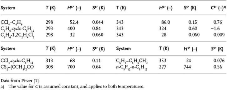
although exceptions do occur. For example, for the system CS₂–CHCl₃, zw (J mol⁻¹) = 5305 − 13.2T, and for the system (C₂H₅)₂O–CHCl₃, zw (J mol⁻¹) = −7368 + 15.5T. These examples make it clear that zw cannot be related to the values for w_ij only, since the w_ij are assumed to be temperature-independent. Experimental thermodynamic values for several systems are given in Table 11.4. Problem 11.15 reveals that the description zw = a + bT is generally insufficient.

Table 11.4 Parameters H^E′ = H^E/Rx₁x₂, S^E′ = S^E/Rx₁x₂ and C^E′ = C^E/Rx₁x₂ for some systems.

Problem 11.10: Regular solution model

Figure 11.3 shows the excess enthalpy H^E for a solution of C₆H₆ in cyclo-C₆H₁₂.

a) Determine the interaction parameter w using the regular solution model assuming a coordination number of z = 10.

b) Calculate the activity coefficient for this solution for x(C₆H₆) = 0.25.

Problem 11.11

Verify Eq. (11.70) and (11.72).

Problem 11.12

A student suggests that the expression for the activity coefficient for one component is given as ln γ₁ = A(1 − x₁)², and that the expression for the second component can be obtained right away by changing the indices. Is this correct?

Problem 11.13

Calculate the vapor pressure for component 2 in a regular solution of 2 in 1.

11.5.3 The Nature of w and Beyond

There remains to be discussed the physical interpretation of the parameter w and how a value for w can be obtained. Let us first discuss the interpretation. In the discussion of the lattice model, we (deliberately) often addressed the parameters w₁₁, w₂₂ and w₁₂ as interactions. Originally, 2w = 2w₁₂ − w₁₁ − w₂₂ was interpreted as the energy (enthalpy) required to create two 1–2 pairs (bonds) from one 1–1 pair and one 2–2 pair. However, it was realized by Guggenheim [2] that w is averaged over all accessible states of the remainder of the system, each weighted with the relevant Boltzmann factor. In this sense, w represents – if taken at constant volume V – the Helmholtz energy, dependent on temperature T and the mole fraction x₁, or – if taken at constant pressure P – the Gibbs energy, again dependent on temperature T and the mole fraction x₁. Of course, the mixing entropy has still to be added. Hence, we can interpret

(11.76)

or, equivalently, turning to molar excess quantities,

(11.77)

as an integral expression for the excess Gibbs energy. Using for the moment w_m(T,P) = N_Aw (T,P) yields , from which we have

(11.78)

A nice illustration is presented by the system CCl₄–C₆H₁₂ for which both G^E and H^E data are available [3], both plotted in Figure 11.5 as a function of x₁x₂. In fact, these data can be described well by the single expression

(11.79)

(11.80)

Figure 11.5 (a) Excess Gibbs energy function G^E and (b) excess enthalpy of mixing H^E for the system carbon tetrachloride and cyclohexane. For clarity, the various curves have been shifted vertically.

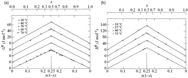
Several other systems obey this approximate relationship (Table 11.4).

Let us now turn to a simple theoretical estimate for w. In the vdW EoS theory, where the parameter a represents the interactions, it was assumed that for mixtures a₁₂ = (a₁₁a₂₂)^1/2. Quantum considerations based on the vdW interaction model indicate indeed, that if some severe approximations are made (see Section 3.6), the interaction energy w₁₂ between molecules 1 and 2 may be approximated⁶⁾ by w₁₂ = −(w₁₁w₂₂)^1/2, where w₁₁ and w₂₂ refer to the interaction energies for the pairs 1–1 and 2–2, respectively. Using this approximation, denoted as Berthelot's rule, we write

(11.81)

This expression is always positive. In this approximation the internal energy change on vaporization for a pure liquid is ΔU₁ = ½N_Azw₁₁, and this provides a basis for estimating w for mixtures of (nonpolar) molecules. This so-called solubility parameter approach will be discussed in Section 11.6 and Chapter 13.

Having discussed the intermolecular interactions in Chapter 3, it seems logical to try to estimate values for w accordingly. We recall Eq. (3.18) reading

(11.82)

where the first term represents the dipolar energy (remember that for an interaction ∼1/T, U = 2F), the second and third terms represent the induction energy, and the fourth term the dispersion energy. One easily obtains, with σ the molecular size, for the dipolar contribution w_dip, the induction contribution w_ind, and the dispersion contribution w_dis,

(11.83)

(11.84)

(11.85)

respectively. Although the order of magnitude of the values obtained is given correctly, the agreement with the experimental values is not particularly striking, while the experimentally observed form zw = a + bT (+ cTlnT) is not reproduced. The reason will be clear: w represents the Gibbs or Helmholtz energy, not the internal energy.

The regular solution model yields symmetric behavior with respect to the two components 1 and 2, although this is not so experimentally in many cases. Moreover, although H^E, S^E and V^E may exhibit complex behavior, G^E is often still rather symmetric and described by G^E = Nzwx₁x₂. There are a number of deficiencies to remedy to go to beyond the regular solution model. First and foremost, there is an inconsistency in the coordination assumptions. We assumed that the coordination is random while there are preferred interactions leading to an interaction enthalpy, and the assumption of random mixing entropy is therefore not correct. However, the correction for this effect appears to be small. Second, the enthalpy estimate is based on nearest-neighbors on a lattice. However, the regular solution model can be freed of the lattice concept, as will be shown in Section 11.6. Further systematic improvement is possible, and some attempts are discussed in Section 11.8.

Although, today, lattice-like models are used less often for small-molecule liquids, they are still instructive because they are simple, and useful because they represent reasonably well the thermodynamics of solutions. Moreover, these models can be systematically improved, which implies that the behavior can be described by just a few parameters. For polymer solutions, lattice models are still extensively used and, of course, simulations can be made more easily nowadays then in the past. Nonetheless, the accuracy of simulations for solutions may still be insufficient.

Problem 11.14

Show that using the heat capacity is .

Problem 11.15

Show that, if zw = a + bT, the parameters a and b relate to the enthalpy and entropy, respectively. Indicate why, considering data from Table 11.4, this description cannot be sufficient. Using zw = a + bT + cTlnT, interpret and estimate a, b and c for the systems CCl₄–C₆H₆ and C₆H₆-cyclo-C₆H₁₂.

Problem 11.16

Verify the expressions for w_dip, w_ind, and w_dis.