Mathematics for the liberal arts (2013)
Part I. MATHEMATICS IN HISTORY
Chapter 4. CALCULUS
4.10 Differential Notation and Estimates
We have grown accustomed to prime notation for derivatives; if f(x) is a function then f′(x) is its derivative. This was the notation of Joseph-Louis Lagrange who lived 1736–1813, and it is one of the most popular derivative notations.
Leonhard Euler (1707–1783) used the capital letter D to indicate derivatives. So the derivative of the function f(x) is Df, or Dxf when we want to be explicit about the dependent variable being x.
Isaac Newton, who lived 1642–1727 and was one of the inventors of calculus, used dot notation. If we recall our example of dropping a pen, we had the position formula
![]()
To indicate a derivative, Newton placed a dot over the dependent variable, y. In his notation, the derivative (which we now know indicates the velocity) looks like
![]()
Gottfried Wilhelm Leibniz, who lived 1646–1716 and is credited along with Newton for the invention of calculus, had yet another notation: differential notation. If y = f(x), then Leibniz’s notation indicates the derivative by the symbol dy/dx.
To understand what Leibniz’s symbol is trying to represent, remember how we came to the idea of derivative. The derivative tells us the slope of a tangent line, and we determine the slope of a tangent line from the slopes of secant lines using a limit.
In normal conversation, we say
![]()
But if we take y = f(x), the “rise” is simply the change in y, which we might write as Δy. Similarly, the “run” is the change in x, or Δx. In this context, the slope of a secant line is
![]()
The slope of the tangent is defined to be the limit of the slopes of the secants over shorter and shorter intervals, that is, the slope as Δx gets closer and closer to 0:
![]()
The Leibniz notation is meant to reflect this process, so
![]()
Where we see Δx and Δy we should think of secant lines. A small change in y is divided by a small change in x. Where we see dx and dy, we should infer tangent lines, i.e., the result of taking a limit.
It is common for people to think of dy/dx as an infinitesimal change in y divided by an infinitesimal change in x. Although this is (formally) a lie, since the real number line is usually not considered to contain infinitesimal values other than 0, it is often a useful and tangible way to think of dy/dx.
Derivatives for Computing Estimates
Derivatives can be useful for estimating small changes in a function. Consider, for example, measuring a square with a ruler. Say we measure the side length to be 5 cm, as in Figure 4.20. Then we know the area to be 25 cm2.
Figure 4.20 Measuring a 5 cm × 5 cm square.
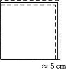
Rulers, however, are not perfect. We never measure a length to be exactly 5 cm. There is always a margin of error. Perhaps we actually know the length to be 5 cm ± 0.1 cm.
Of course, a change in the side length means a corresponding change in the area of the square. We can compute this directly: the largest possible area is 5.1 cm × 5.1 cm = 26.01 cm2, and the smallest is 4.9 cm × 4.9 cm = 24.01 cm2.
We can also estimate this in a calculus context by letting x represent the length of the side we are measuring so that y = f(x) = x2 is the area. Our goal is to estimate the change in f(x) that comes from changing (or mis-measuring) xby a small amount.
We’ve emphasized that the derivative is a limit of slopes of secant lines. Another way of saying this is that when Δx is small, the slope of the secant is approximately the same as the slope of the tangent. When Δx is small,
![]()
Multiplying by Δx, we get a formula that estimates the change in the function.
The derivative approximation rule: ![]() .
.
In our case, since y = f(x) = x2, we have dy/dx = 2x. We measured x = 5 cm, but we may have a measurement error as large as Δx = ±0.1 cm. To estimate the error in the area, we compute:
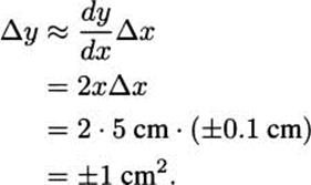
So, we estimate the area of the square to be 25 cm2 ± 1 cm2 ; it may be as low as 24 cm2 or as high as 26 cm2. This estimate matches almost exactly what we obtained by direct computation.
To understand how this estimate works, it may help to look carefully at the graph of f(x) = x2 near the point x = 5.
Figure 4.21 The function f(x) = x2 near x = 5.
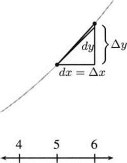
In this picture, Δy indicates the true change in the value of a function, the true difference that we could compute by evaluating the function at two points and subtracting. For example, if this is the graph of y = x2 with Δx = 1, then Δy = 36 – 25 = 11.
The value dy is the corresponding change that happens in the tangent line. We know from the derivative that the slope at 5 is f′(5) = 2 · 5 = 10, so the equation of the tangent line (in point-slope form) is y – 25 = 10(x – 5), or in the slope-intercept form, y = 10x – 25. Evaluating at x = 6 and x = 5, we subtract to get dy = 35 – 25 = 10. This is a bit smaller than the true Δy of the function, and we can see this on the graph.
We took Δx = 1 cm, a pretty large change. Imagine how much closer the estimate would be if we took Δx = 0.1 cm. The difference between Δy and dy would be very small. This is the key to approximating with derivatives. For small changes in x, the tangent line is a close approximation to the function, so (vertical) changes measured on the tangent line do a good job of estimating (vertical) changes in the function.
The symbol dy is called the differential of the function. This is why the symbol dy/dx is often referred to as differential notation and why the method of approximating with derivatives is called differential approximation.
![]() EXAMPLE 4.28
EXAMPLE 4.28
Estimate ![]() using only the operations available on a 4-function calculator.
using only the operations available on a 4-function calculator.
Solution: If we let f(x) = ![]() , then our task is to estimate the value of f(8.95). Fortunately, the value f(9) = 3 is easy to calculate. We can apply a differential approximation using Δx = –0.05 to see how much f changes as we move to the nearby x-value:
, then our task is to estimate the value of f(8.95). Fortunately, the value f(9) = 3 is easy to calculate. We can apply a differential approximation using Δx = –0.05 to see how much f changes as we move to the nearby x-value:
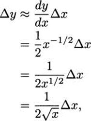
and using x = 9 and Δx = –0.05, we get
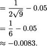
Having estimated the change in function value, we can now calculate that ![]()
![]() – 0.0083 = 2.9917. We used only addition, subtraction, multiplication, and division (the operations available on a 4-function calculator).
– 0.0083 = 2.9917. We used only addition, subtraction, multiplication, and division (the operations available on a 4-function calculator).
![]()
It may have never occurred to you, but even powerful computer chips often know how to do only simple operations. More complicated calculations, such as roots and the values of trigonometric functions, are typically produced by approximation methods programmed in software.
EXERCISES
4.49 The side length of a cube is measured to be x = 15 cm with a margin of error of ±0.5 cm. Estimate the change in the volume that results from measurement error.
4.50 The side length of a cube is measured to be x = 15 cm with a margin of error of ±0.5 cm. Estimate the change in the surface area that results from measurement error.
4.51 The radius of a circle is measured to be r = 30 cm with a margin of error of ±1 cm. Estimate the change in area that results from measurement error.
4.52 The radius of a sphere is measured to be r = 30 cm with a margin of error of ±0.1 cm. Estimate the change in volume that results from measurement error.
4.53 The Earth is approximately spherical, with a radius of 6378.1 km. A ‘belt’ of 40074.8 km would wrap around the “waist” of the Earth. If 1 m of slack were added to the belt, how high would the belt rise above the Earth? (Hint: you are given a circumference C with change ΔC, and asked to estimate Δr.)
4.54 The Moon has a ‘waist size’ of 10916.4 km. If 1 m of slack were added to its ‘belt,’ how high would the belt rise above the surface of the Moon?
4.55 Use differential approximation to estimate each value:
a) ![]()
b) ![]()
c) ![]()
d) ![]() (Hint: 100/49 is a perfect square.)
(Hint: 100/49 is a perfect square.)
e) ![]() (Hint: find a ratio of perfect squares near the value 5.)
(Hint: find a ratio of perfect squares near the value 5.)