Liquid-State Physical Chemistry: Fundamentals, Modeling, and Applications (2013)

In this appendix we review briefly the lattice gas model [1], which is widely used in physical chemistry and known under different names in various fields, for example, as the regular solution model for liquid solutions, as the order–disorder model for alloys [2], or as the Ising model [3] for magnetic problems [4]. This broad range of applications explains its importance. For pure liquids the model was introduced by Frenkel [5] in 1932, and somewhat later independently by Eyring (and Cernuschi) [6]. It is one of the simplest models, if not the simplest model, showing a phase transition¹⁾, but we should note here that, although the model looks deceptively simple, its solution is complex.

C.1 The Lattice Gas Model

The basic idea of the lattice gas model is that the volume available to the fluid is divided into cells of molecular size. Usually, for simplicity, the cells are arranged in a regular lattice with coordination number z, for example, a simple cubic (SC) lattice with z = 6, a body-centered cubic (BCC) lattice with z = 8, or a face- centered cubic (FCC) lattice with z = 12. Normally, these cells are occupied by one molecule at most, representing repulsion, and only nearest-neighbor cell attractive interactions are considered.

The lattice gas model can be solved exactly for 1D, and in this case the model does not show a phase transition. It can also be solved exactly for 2D without an applied field, as was achieved for the first time by Onsager [7]; in this case, the model does show a phase transition. A complete exact solution (i.e., with applied field) is neither known for 2D, nor for 3D, so that one has to approximate. We will not deal with the exact 2D solution [2] but discuss here first the (conventional) zeroth approximation or mean field solution²⁾ in terms of a model for liquid solutions, and thereafter the first approximation or quasi-chemical solution. In fact we have used these approximations in Chapters 8 and 11 already, although expressed in slightly different terms.

C.2 The Zeroth Approximation or Mean Field Solution

For a lattice model of a liquid solution we distribute molecules of type 1 and type 2 over the lattice (without any further holes). In Section 8.3, we showed that if we have N₁ molecules of type 1 with N₂ molecules of type 2, so that the total number becomes N = N₁ + N₂, we obtain the general relations

(C.1)

while the energy is given by

(C.2)

Here N₁₁ (N₂₂, N₁₂) represent the number of type 1–1 (2–2, 1–2) pairs, ε₁₁ (ε₂₂, ε₁₂) the energy of the pair 1−1 (2−2, 1−2), and the quantity w ≡ ε₁₂ − ½ε₁₁ − ½ε₂₂ is denoted as interchange energy. To be consistent with Section 8.3 and Chapters 8 and 11, we use the notation zX ≡ N₁₂, so that

(C.3)

The canonical partition function is easily constructed and we obtain

(C.4)

Recognizing that the term B ≡ ½(zε₁₁N₁ + zε₂₂N₂) is constant, this reduces to

(C.5)

where the sum Σ_{X} is over all configurations having X type 1–2 pairs and q_j is the internal partition function of molecule j. Equivalently, we write

(C.6)

where the sum Σ_X is now over the number of configurations having X type 1–2 pairs with the degeneracy factor g(N₁,N₂,X) for each configuration labeled with (N₁,N₂,X).

In the zeroth approximation we consider that molecules are distributed randomly over the lattice, in spite of their interaction with others, which we restrict to their z nearest-neighbors. For the number of type 1–2 pairs zX we then get

(C.7)

(C.8)

The first expression was used in Chapter 8, but here we will use the second expression. The next step is to calculate g(N₁,N₂,X). Considering the distribution N₁ molecules of type 1 and N₂ of type 2 over N cells, one obtains for the number of configurations

(C.9)

Therefore, the partition function becomes

(C.10)

so that for the Helmholtz energy the result is

(C.11)

(C.12)

Consequently, the mixing Helmholtz energy reads

(C.13)

As a check, one can calculate the internal energy of mixing Δ_mixU energy from Δ_mixF via U = ∂(F/T)/∂(1/T) which leads, as expected, to

(C.14)

The coexistence line between a phase-separated system and a homogeneous system can be calculated from ∂Δ_mixG/∂x₂ = ∂Δ_mixF/∂x₂ = 0. This leads to

(C.15)

Using the transformation s = 2x₂ − 1, the final expression is

(C.16)

The critical temperature T_cri is the temperature where the molecules start to order, and we determine T_cri by considering that tanh(½βzws) is a continuously increasing function of s passing through s = 0. Hence, there is always the solution s = 0 but for d[tanh(½βzws)]/ds|_s=0 > 1, two other solutions occur (Figure C.1). Because this derivative equals ½βzw, we find T_cri = zw/2k. The composition as a function of T can be found by solving Eq. (C.16), either numerically or graphically, and the result is shown in Figure C.2a.

Figure C.1 The curves y = s and y = tanh(as) with (a) a = 0.5, (b) a = 1.0, and (c) a = 2.0, showing for the zeroth order solution, respectively, the homogeneous state (T > T_cri), the critical state (T = T_cri), and the phase-separated state (T < T_cri). All curves are plotted for s ≥ 0 only.

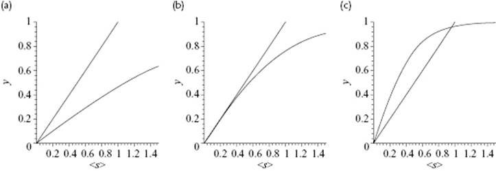
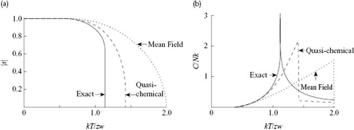
Figure C.2 The composition |s| = |2x₂ − 1| where phase separation occurs (a) and the associated heat capacity C/Nk (b) as a function of kT/zw for the 2D square lattice, showing the zeroth order (mean field), the first order (quasi-chemical), and the exact solution.

The associated heat capacity C_V can be found from C_V = ∂U/∂T, with resulting in (after some calculation and plotted in Figure C.2b)

(C.17)

Note that C_V shows a finite jump at T = T_cri with a maximum of 3Nk.

C.3 The First Approximation or Quasi-Chemical Solution

In the zeroth approximation, single molecules are distributed independently and randomly over the lattice. Improvement is possible by distributing randomly pairs of molecules instead of single molecules. This solution is known as the first approximation or quasi-chemical solution³⁾.

C.3.1 Pair Distributions

Let us consider an independent distribution of pairs 1–1, 1–2, 2–1 and 2–2 over the lattice. Any such a distribution is characterized by the numbers N₁, N₂ and X, and this leads in the usual way to the number of possible configurations

(C.18)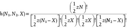

where we have used a separate entry for the 1–2 and 2–1 pairs in order to avoid the use of a symmetry number. This result cannot be correct, as the sum over all configurations zX should yield N!/N₁!N₂!. However, we can − at least approximately − remedy this defect by introducing a normalization factor c(N₁,N₂), and write for

(C.19)

(C.20)

We evaluate the sum G by taking its largest term (see Justification 5.2), and this term, labeled by X*, is obtained by setting ∂G/∂X = 0. The result is, after some straightforward manipulation,

(C.21)

This implies that the sum G for X*, labeled G*(N₁,N₂), becomes

(C.22)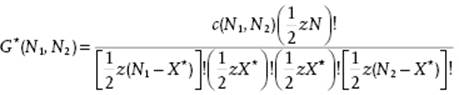

If we sum g(N₁,N₂,X) over all values of X, we must regain the total number of ways of placing N₁ molecules of type 1 and N₂ of type 2 over N = N₁ + N₂ sites. In other words, we also have G = N!/N₁!N₂! and we obtain for c(N₁,N₂)

(C.23)

Therefore, g(N₁,N₂,X) = N!h(N₁,N₂,X)/N₁!N₂!h(n₁,n₂,X*) or, in full

(C.24)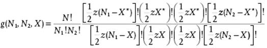

The configurational partition sum Q becomes

(C.25)

with, as usual, β = 1/kT. The maximum term trick is now played again and hence we seek the maximum term of Q, labeled , by setting ∂Q/∂X = 0, or equivalently, by setting ∂lnQ/∂X = 0. After a straightforward calculation we obtain

(C.26)

For an explicit solution we define η² ≡ exp(2βw) and the parameter α by

(C.27)

so that we can transform Eq. (C.26) to α² − (1 − 4x₁x₂) = 4η²x₁x₂ (or α² − (1 − 2x₂)² = 4η₂x₁x₂), which has the solution α = [1 + 4x₁x₂(η² − 1)]^1/2 with x_j = N_j/(N₁ + N₂). The energy of mixing becomes Δ_mixU = 2x₁x₂zwN/(α + 1). Note that for α = 1 we regain the zeroth approximation.

C.3.2 The Helmholtz Energy

The configurational Helmholtz energy F is given by F = −kTlnQ and becomes

(C.28)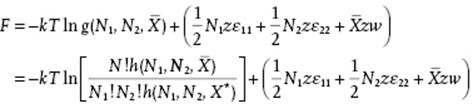

The evaluation of F is complex, and it is convenient to calculate first the chem­­ical potential μ_j = ∂F/∂N_j. If this calculation is handled without thinking, it is a straightforward but tedious task. However, if we realize that is obtained from , the evaluation becomes straightforward. This implies that all terms resulting from taken together cancel. Moreover, X* is obtained from ∂lng/∂X = 0, implying that all terms from ∂lng/∂X* taken together also cancel. This renders the differentiation of F a relatively simple task, leading to

(C.29)

To obtain μ_j − μ_j°, we realize that μ_j° is obtained from Eq. (C.28), again via μ_j = ∂F/∂N_j, but now with N₂ = 0, leading to μ_j° = ½zβε_jj. Writing F = N₁μ₁ + N₂μ₂ = N(x₁μ₁ + x₂μ₂), we obtain for the molar Helmholtz energy of mixing

(C.30)

Using the (absolute) activity λ_j = exp(βμ_j) and, as before, assuming that the activity can be replaced by the partial pressure, the activity coefficient γ becomes

(C.31)

In all these expressions X* and are given by Eq. (C.21) and (C.27), respectively.

C.3.3 Critical Mixing

The above expression for Δ_mixF_m can be made more explicit by writing the various contributions in terms of α = [1 + 4x₁x₂(η² − 1)]^1/2 with η² ≡ exp(2βw), x₁ = N₁/(N₁ + N₂) and x₂ = N₂/(N₁ + N₂). We find

(C.32)

(C.33)

(C.34)

so that Δ_mixF_m becomes

(C.35)

A similar substitution can be made for and P_j, leading to

(C.36)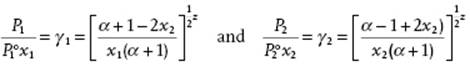

The critical point, due to symmetry, still occurs at x₁ = x₂ = ½. To obtain the expression for T_cri, we first derive the expression for the coexistence line, determined by . Upon substitution of the expression for we obtain

(C.37)

where the molecular ratio r ≡ x₂/x₁ and the abbreviation γ are introduced. Solving α yields α/(1 − 2x₂) = (1 + γ)/(1 − γ), and thus leads to

(C.38)

Multiplying these two expressions leads to

(C.39)

Comparing with the transform of Eq. (C.26), α² − (1 − 2x₂)² = 4η²x₁x₂, we obtain

(C.40)

Note that if r = r₁ is a solution of Eq. (C.36), the other one is r₂ = 1/r₁.

The critical temperature T_cri is now obtained by putting r = 1 + δ in Eq. (C.40), expanding in powers of δ and taking the limit δ → 0. We thus obtain

(C.41)

For the SC lattice (z = 6) we have zw/kT_cri = 2.433, while for the BCC lattice (z = 8) and FCC lattice (z = 12) we obtain zw/kT_cri = 2.301 and zw/kT_cri = 2.188, respectively. Note that if we take z = ∞, we regain the zeroth approximation zw/kT_cri = 2.

Calculating, as before, the internal energy via U = ∂(F/T)/∂(1/T) is considerably more complex as for zeroth approximation and leads to

(C.42)

So far w was considered to be temperature independent but considering w as a temperature-dependent parameter presents no specific problems, and by using the definition u ≡ w − T(∂w/∂T), one can show that in this case one obtains Δ_mixU = 2Nzux₁x₂/(α + 1).

C.4 Final Remarks

As stated in Section C.2, only a (partial) exact solution exists for 2D lattices. For a square lattice this solution reads zw/kT_cri = 3.523, to be compared with zw/kT_cri = 2.773 for the first and zw/kT_cri = 2.00 for the zeroth approximation. The results from the exact solution for s and C_V are shown, as are the results for the zeroth and first approximation, in Figure C.2. From these plots it becomes clear that considerable improvement is obtained by using the first approximation, but also that the exact solution is still far from being approached. Finally, the higher the number of dimensions, the better the mean field solution (see Chapter 16), which implies that the situation for 3D is somewhat better than for 2D.

Notes

1) For a very readable introduction to phase transitions, see Ref. [8].

2) Also denoted as the Bragg-Williams approximation.

3) Also denoted as the Bethe–Peierls approximation. For further details, see Refs [9] and [10].

References

1 Yang, C.N. and Lee, T.D. (1952) Phys. Rev., 87, 404 and 410.

2 Huang, K. (1987) Statistical Mechanics, 2nd edn, John Wiley & Sons, Inc., New York.

3 Ising, E. (1925) Z. Phys., 31, 253.

4 Brush, S.G. (1967) Rev. Mod. Phys., 39, 883.

5 Frenkel, J. (1946) Kinetic Theory of Liquids, Oxford University Press, Oxford. See also Dover Publishers reprint (1953).

6 (a) Eyring, H. (1936) J. Chem. Phys., 4, 283; (b) Cernuschi, F. and Eyring, H. (1939) J. Chem. Phys., 7, 547.

7 Onsager, L. (1944) Phys. Rev., 65, 117.

8 Stanley, H.E. (1971) Introduction to Phase Transitions and Critical Phenomena, Oxford University Press, New York.

9 Fowler, R.H. and Guggenheim, E.A. (1939) Statistical thermodynamics, Cambridge University Press.

10 Guggenheim, E.A. (1952) Mixtures, Clarendon, Oxford.