Liquid-State Physical Chemistry: Fundamentals, Modeling, and Applications (2013)

3.7. Refinements

In this section we introduce hydrogen bonding and three-body interactions, and deal briefly with in how far empirical potentials are accurate.

3.7.1 Hydrogen Bonding

All of the above-mentioned interactions are generally valid. There is, however, a special bond, designated as hydrogen bond, which is an attractive interaction between two electronegative species A and B that form a link A−H···B via the covalently bonded H-atom and the lone pair of electrons (or polarizable π electrons) of B. The Lewis acid A withdraws some charge form the H-atom, leading to a partial charge δ⁺ which interacts with δ⁻ of the Lewis base B. It is often said that this type of bonding is restricted to F, O and N atoms, but other species, such as negative ions (anions), can also participate in hydrogen bonding. For the F, O and N atoms, the interaction strength decreases from the F–H to the O–H to the N–H bond.

The hydrogen bond can also be considered as a delocalized bond in which orbitals from the A and B species as well the 1s orbital of the H atom are involved and which accommodates four electrons (two electrons from the A–H bond and two from the lone pair of atom B). These four electrons occupy the two lowest molecular orbitals, leading to an overall energy lowering. Since the hydrogen bond, of which the strength is typically about 10–40 kJ mol⁻¹, is based on orbital overlap, its strength decreases rapidly with distance. However, when this type of bonding is active it is often dominating over the other van der Waals interactions. Two types of hydrogen bond can be distinguished, namely, an intramolecular bond between A and B atoms within the same molecule, and an intermolecular bond between A and B atoms from different molecules. An example of the former is found in ortho-hydroxybenzoic acid, while the latter occurs, for example, in H₂O and CH₃COOH.

The hydrogen atom in the O–H···O bond has two nonequivalent minimum energy positions, each near each of the two O atoms, separated by an energy barrier. The O–H bond (typically ∼0.097 nm) is shorter than the H···O bond (0.25–0.28 nm). The enthalpy of dissociation is typically 12–25 kJ mol⁻¹, but carboxylic acids in the gas-phase form an exception with ∼30 kJ mol⁻¹. Hydrogen bonds provide multiple options for bonding in water, which leads to a residual entropy for ice of R ln(3/2) and anomalous behavior of water (e.g., low compressibility, high permittivity and a minimum density at 4 °C; see Chapter 10). Hydrogen bonding also leads to a number of other phenomena deviating from expected, normal behavior; for example, when hydrogen bonding is present significant deviations occur from Trouton's rule and Eötvös' rule⁹⁾. Clearly, the infrared frequencies of the OH bond are influenced by the presence of a hydrogen bond. For example, for gaseous water the bond is characterized by a wave number of ∼3756 cm⁻¹, whereas for liquid water the wave number decreases to ∼3453 cm⁻¹. While the O–H···O hydrogen bond plays an important role in water, bonds of the type N–H···O=C occur in, for example, urea and proteins, playing important roles in biological systems.

In a simple model for collinear O–H···O bonds, the O–H···O bond energy ϕ_H-bond can be described by a Morse potential for the O–H bond with distance r and one for the H···O bond with distance R−r, plus the interaction between the two O atoms, u(R). This expression contains several parameters: the bond dissociation energies ε₀; the force constants a₀ for these bonds unperturbed and their associated equilibrium distances r₀; the distance between the two O atoms R; and, finally, the parameters in the function u(R). The values for these parameters can be obtained from the condition (∂ϕ_H-bond/∂r)_eq. = 0. The IR shifts Δν = ν_H-bond − ν₀, with ν₀ the unperturbed bond frequency, are obtained from the force constant a = (∂²ϕ_H-bond/∂r²)_eq., and are to be compared with the experimental data.

Hydrogen bonding affects properties to a considerable degree, but two examples will suffice at this point. Ethanol (CH₃CH₂OH) and dimethyl ether (CH₃OCH₃) are of similar size and have the same number of electrons; moreover, their dipole moments are not very different. Nevertheless, their boiling points are 78.5 °C and −24.8 °C, respectively. Pentane (C₅H₁₂) and butanol (C₄H₉OH) are also of similar size and have the same number of electrons, but in this case the dipole moment of butanol aids to increase the intermolecular interaction (C₅H₁₂ is apolar) and their boiling points are 36.3 °C and 117 °C, respectively. The field of hydrogen bonding is rich and elaborate. A classical review has been provided by Pimentel and McLellan [8] while Grabowski [9] provides a more recent review.

3.7.2 Three-Body Interactions

So far, we have been discussing intermolecular interactions in terms of two-body potentials. However, there is no reason why a third body would not influence the interactions between two bodies, apart from contributing to the sum of the two-body potentials for all three bodies. The dipolar three-body interaction is probably [10] the most important, and has been studied by Axilrod and Teller [11] along the lines of the van der Waals potential for two bodies, resulting in

Here, θ₁ denotes the internal angle between the vector with length r₁₂ between particles 1 and 2, while r₁₃ is the length of the vector between particles 1 and 3. The angles θ₁ and θ₃ have a similar meaning, and the sign of this contribution depends on the geometry of the triangle formed. For acute triangles ϕ₁₂₃ > 0, whereas for obtuse triangles ϕ₁₂₃ < 0. The significance of the three-body interaction has been estimated rather differently by various authors. On the one hand, Rowlinson [12] indicated a too-negative potential energy by “10–15% of the total potential energy of a normal liquid,” alleviating this to 5–10% for a typical configuration in a liquid where most close triplets of molecules form acute-angled triangles, but also indicating a substantial cancellation of multibody terms. Dymond and Alder [13], on the other hand, indicated a contribution “… as little as 1–2%,” supported by Berendsen [14], who stated that the contribution is probably negligible. Here, attention will be paid to three-body interactions only occasionally.

3.7.3 Accurate Empirical Potentials

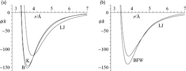
Although model potentials are useful, they are idealized. Figure 3.5 shows a typical set of curves for Ar [15] fitted on second virial coefficients over a temperature range of −190 °C to 600 °C. It is clear that both the depth and location of the potential vary considerably with the type of potential. Similar differences are obtained for other molecules. A rather complete evaluation on Ar dimers has been given by Parson et al. [16]. Only for a few cases are accurate empirical potentials available, the inert gases being such a case. Barker and coworkers [17] represented the Ar potential as a sum of pair potentials and the Axilrod–Teller three-body interaction resulting in a 15-parameter equation (!). For fitting, they used the thermodynamic and transport data of the gas, the low temperature properties of the solid, the internal energy and self-diffusion coefficient of the liquid, and the equation of state. This provided an excellent agreement with the vibration spectrum of bound Ar dimers, and with molecular beam scattering cross-section determinations [16]. It appeared also to describe the solid-state internal energy, the elastic constants, the phonon curves, and the solid-fluid coexistence curve well. Calculations of the third virial coefficient with this potential showed the contribution of the three-body interaction to be quite significant, and to bring the theoretical results into good agreement with the experimental data. Figure 3.5 shows a comparison with the optimum Lennard-Jones potential, indicating that the latter is shallower at its minimum and longer-ranged than the optimum potential. On the other hand, simple pair potential calculations for the condensed phase perform quite well in practice. So, it might be wondered why these potentials do not perform very badly. Barker et al. concluded that the three-body effects partially cancel out in the condensed phase, and that three-body effects are taken into account in an averaged way by using a fitted two-body potential. However, their studies showed that a single potential for Ar derived from bulk data is capable of describing all properties.

Figure 3.5 (a) Comparison of the Lennard-Jones (LJ), Kihara (K), and Buckingham (B) potential for Ar, showing the difference in minimum and depth of the various potentials; (b) Comparison of the Lennard-Jones (LJ) and Barker–Fisher–Watts (BFW) potential for Ar, showing that the LJ potential is more shallow at its minimum and longer ranged than the BFW potential.

Problem 3.18

Estimate the relative contribution of the three-body interaction for a triplet of Ar atoms arranged in an equilateral triangle. Use data from Table 3.1.