Liquid-State Physical Chemistry: Fundamentals, Modeling, and Applications (2013)
3. Basic Energetics: Intermolecular Interactions
3.6. Model Potentials
Although the above given description provides an insightful description of the intermolecular interactions, a more simple potential is often required. It is clear that any simplified potential should contain an attractive part and a repulsive part. However, the simplest potential that can be used is the hard-sphere (HS) potential, given by
(3.21) ![]()
where σ is the hard-sphere diameter. Although highly artificial, this potential is nevertheless often used in simple models and as a reference potential.
The simplest way to improve and include attractive interaction to the hard-sphere potential is to add a region with a constant attraction. This leads to the square-well (SW) potential given by
(3.22) 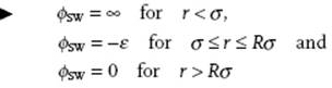
where, as before, σ is the hard-sphere diameter and ε and Rσ are the depth and range of the square-well, respectively. Typically, the value of R is ∼1.5–2.0, and although simple it will appear to be versatile.
A more realistic expression is the Mie potential given by
(3.23) ![]()
where b, c, n and m are parameters and n > m. An often-used choice, mainly for convenience, is the 12-6 or Lennard-Jones (LJ) potential with n = 12 and m = 6. In this case, an alternative form for Eq. (3.23) is
(3.24) ![]()
Here, the parameter ε describes the depth of the potential energy curve, while r0 is the position of the minimum. For the LJ 12-6 potential we thus have r0 = 21/6σ, ϕLJ(r0) = −ε, and ϕLJ(σ) = 0. The parameter σ can be seen as the diameter of the molecule. The LJ potential describes the interaction energy qualitatively rather well (Figure 3.1). Typical values of parameters for the LJ potential for some molecules are given in Appendix E. It is clear that slightly different values will be obtained, depending on which properties and procedures are used for their evaluation.
For quasi-spherical molecules, such as SF6, CF4 and C(CH3)4, both the attractive and repulsive forces decrease more rapidly than would be expected from the Lennard-Jones potential. This implies a higher value for both the exponents 12 and 6. In fact, we can write the Mie potential, using ε and r0, as
(3.25) ![]()
The potential for quasi-spherical molecules can be described by (n,m) = (28,7), where the precise choice is largely dictated by mathematical convenience. An alternative for quasi-spherical molecules is the Kihara potential [3], which describes the interaction in a similar way as the Lennard-Jones potential but includes a hard core. It is given by
(3.26) ![]()
where δ is the diameter of the hard core. We thus have ϕK(r < δ) = ∞ and ϕK(σ) = 0. Typical values for δ are δ/σ = 0.084 for Ar, 0.194 for N2, 0.655 for C6H6, and 0.900 for n-C6H14. The shape as a function of distance resembles that of the Mie 28-7 potential, taking δ equal to one-quarter of the van der Waals radius [4].
While the power-law relationship with m = 6 can be rationalized for the attractive part of the potential, the repulsion is on quantum-mechanical grounds expected to be better described by an exponential. This leads to the Buckingham or exp-6 potential
(3.27) ![]()
where ε, r0, and α are parameters, representing dissociation energy, equilibrium distance, and (scaled) force constant, respectively. Because this potential shows a maximum at a small value of r, the condition ϕB = ∞ for r < rmax is added. Another often-used expression is the Morse potential [5] given by
(3.28) ![]()
with ε, r0, and α parameters.
For estimates of the interaction between unlike molecules, we limit ourselves to the r−6 attraction. The repulsion is usually modeled as for hard-spheres, that is, we use for spheres i with diameter σii the combination rule σij = (σii + σjj)/2, often denoted as the Lorentz rule. For the attraction we learned from the London treatment that
(3.29) ![]()
Comparing this expression with the attractive part of the LJ potential
(3.30) ![]()
results in
(3.31) ![]()
Substitution of Ii in Eq. (3.29) yields after some manipulation
(3.32) ![]()
Since reliable information on I is scarce, this is a clever way, essentially proposed by Kohler [6], to circumvent the need for an estimate of I.
If we take σii = σjj and Ii = Ij, we obtain the geometric mean εij = (εiiεjj)1/2, often denoted as the Berthelot rule. However, while the Lorentz rule is quite acceptable, the Berthelot rule is only very approximate. From a sensitivity analysis for ε12 using the Lorentz–Berthelot rule it appears that the ratio σ11/σ22 has a particularly large influence. Nevertheless, if intermolecular interactions are fitted to experimental data, the Lorentz–Berthelot rule is frequently used. It is clear that the success of Berthelot's rule is fortuitous and due to the partial canceling of errors.
Problem 3.12
Show that r0 = 21/6σ, ϕLJ(r0) = −ε and ϕLJ(σ) = 0.
Problem 3.13
Show that the force constant a for the Morse and Kihara potential are given by ![]() , respectively.
, respectively.
Problem 3.14
Another well-known potential is the so-called universal bonding curve [7]
![]()
Show that the force constant a for this potential a = ε/l2, neglecting the x3 term.
Problem 3.15
Show that, if σ11 = σ22 and I1 = I2, Eq. (3.32) yields ε12 = (ε11ε22)1/2 and that ε12 < (ε11ε22)1/2 otherwise.
Problem 3.16
Estimate ε12 using ε12 = (ε11ε22)1/2 as well as the more complete expression [Eq. (3.32)], taking a typical value of α1′/α2′ = 2 for values of σ11/σ22 and ε11/ε22 ranging from 1 to 2. How do you assess the quality of the Berthelot rule?
Problem 3.17
Show, assuming εcoh = −A/r6, that the average molecular cohesive energy of a fluid is given by
![]()
Do so, assuming a random distribution of N molecules over a volume, that is, a uniform number density ρ = N/V, by integrating εcoh for a reference molecule over a spherical shell for the smallest distance of approach σ to some macroscopic distance R. By taking this interaction over all pairs of molecules, show that the total molar cohesive energy Ucoh reads
![]()
Estimate the value of Ucoh for CCl4 with mass density ρ′ = 1.59 g cm−3 and molecular mass M = 153.8 g mol−1. Do so on the one hand by estimating σ from the polarizability volume α′ and A from Eq. (3.18), and on the other hand from the LJ parameters ε and σ leading to A = 4εσ6, and comment on the agreement with the experimental value Ucoh = 32.8 kJ mol−1.