Corresponding States - Describing Liquids: Phenomenological Behavior - Liquid-State Physical Chemistry: Fundamentals, Modeling, and Applications (2013)

Liquid-State Physical Chemistry: Fundamentals, Modeling, and Applications (2013)

4. Describing Liquids: Phenomenological Behavior

4.3. Corresponding States

The CP is characterized by (∂P/∂V)_T = (∂²P/∂V²)_T = 0, and this leads for the vdW equation to (with V the molar volume V_m)

(4.7)

Defining the reduced quantities

(4.8)

we can write the EoS in a nondimensional form, usually called the reduced vdW equation of state, and given by

(4.9)

As this reduced equation contains no constants characteristic of a particular fluid, the result is (theoretically) valid for all fluids, and represents an example of the principle of corresponding states (PoCS). Quite apart from the applicability of the reduced vdW EoS, the PoCS is an experimental fact which asserts that, for a group of similar substances, the EoS can be written in the form

(4.10)

where Ω is the same function for all the substances of the group.

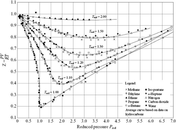
In order to estimate a and b, the values P_cri and T_cri (see Appendix E) can be used. Another way of determining a and b is to fit P to the vdW equation for a range of temperatures. It will be clear that different procedures yield (slightly) different values. The (approximate) validity of the PoCS is indicated by the fact that the compression factor at critical conditions Z_cri = P_criV_cri/RT_cri is approximately constant for a set of spherical, nonpolar molecules at (0.293 ± 0.005), where ± indicates the sample standard deviation (Table 4.3). Note that for the vdW fluid Z_cri = 3/8 = 0.375. Perhaps more convincing is a plot of Z versus P_red, as given in Figure 4.4 for several molecules, which shows that the curves for a certain, fixed T_red nicely coincide.

Table 4.3 Critical reduced compression factor and surface tension for several simple molecules.

c4-tbl-0003

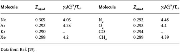
Figure 4.4 Compression factor Z as a function of the reduced pressure for various fluids, illustrating the principle of corresponding states. Data from Ref. [17].

c4-fig-0004

Another example of the PoCS is shown in Figure 4.5, where the second virial coefficient B/V_cri versus T/T_cri for Ar, Kr, Xe and CH₄ is shown. The curve can be described well by the expression as derived for the square-well potential (see Chapter 3) with a hard-core diameter σ, a depth ε and a range 1.5σ, and is given by

(4.11)

Figure 4.5 (a) The common curve of T/T_cri versus ρ/ρ_cri for various fluids; (b) The common curve of B/V_cri versus T/T_cri for Ar, Kr, Xe, and CH₄. Both curves represent examples of the PoCS.

c4-fig-0005

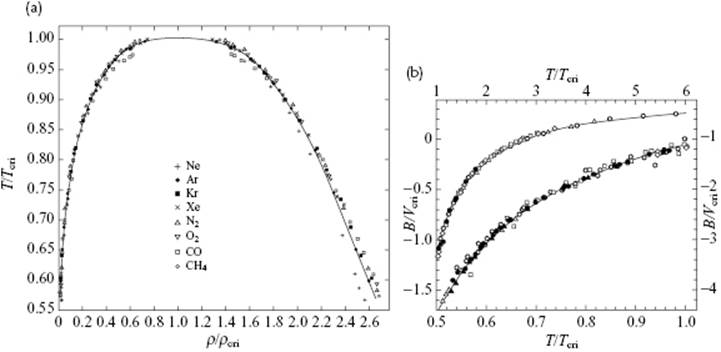
The parameters σ and ε are given by ⅔πN_Aσ³ = 0.447V_cri and ε = 0.936kT_cri. As a final example, Figure 4.5 also shows ρ/ρ_cri versus T/T_cri. The curve is well fitted by

(4.12)

where ρ_L and ρ_G represent the densities of the liquid and gas, respectively. The first of these expressions represents the law of rectilinear diameters, which states that the average density of gas and liquid is a linear function of its temperature.

The PoCS implies that the intermolecular potential has a similar shape for the molecules within the class of molecules considered. For a two-parameter intermolecular potential of the form ϕ(r) = εf(r/σ), the distances are scaled by σ, while the energy is scaled by ε. Consequently, we can scale the pressure P according to P* = σ³P/ε, the volume V according to V* = V/σ³, and the temperature T according to T* = kT/ε. Finally, the configurational partition function (see Chapter 5) scales according to Q* = Q/σ^3N. In this way, the pressure becomes

(4.13)

In this dimensionless representation, the P–V curves of a set of molecules should coincide for the same T*, as illustrated in Figure 4.4 using T_red.

4.3.1 Extended Principle*

The conventional corresponding state approach deals with two parameters, for example, using the compression factor Z = Z(T_red,P_red). For simple, (more or less) spherical molecules this approach works reasonably well, as evidenced by the “universal” value of the compression factor Z [3]. In fact, any EoS that contains only two parameters can be mathematically reduced likewise. However, the reduction is essentially based on dimensional analysis with force, length and temperature as basic dimensions. In the case of categories of molecules for which extra dimensions are important, one does not expect the principle to apply. A significant improvement in describing experimental results can be obtained by extending the concept to three parameters, of which the best known approaches are due to Riedel [4] and Pitzer [5]. Both approaches use the pressure P versus temperature T. Riedel used the parameter α = (d lnP/d lnT)_T_=Tcri taken along the saturation curve, while Pitzer et al. used a parameter that can be obtained if we plot the logarithm of the saturated vapor pressure in reduced units versus 1/T_red. In this representation, approximately straight lines are obtained, that is, . 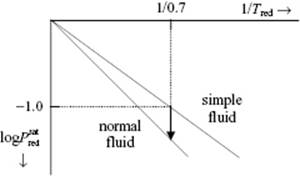The two-parameter principle predicts that the slope S is the same for all substances. If we plot the vapor pressures of simple fluids (spherical molecules such as Ar, CH₄, …), they indeed all fall more or less on the same line that appears to go through at T_red = 0.7. However, other, less-spherical molecules do have different slopes. These facts are used to define the so-called acentric factor (Figure 4.6). This apparently arbitrary definition was chosen because of the ease and precision with which this quantity can be determined (contrary to Riedel's α, which might be difficult to determine precisely). Since at T/T_cri = 0.7 the vapor pressure of simple fluids is close to 0.1 P_cri, the acentric factor is essentially zero for these compounds. The relation of the acentric factor ω to Riedel's α reads ω = 4.93(α − 5.808), and therefore we limit ourselves further on to ω. The acentric factor ω is given for a variety of compounds in Appendix E [6].

Figure 4.6 The acentric factor ω as the deviation of the slope of the vapor pressure of a normal from the fluid slope for simple fluids. Note: log = logarithm to base 10.

c4-fig-0006

The simplest correlation [7] for normal fluids is

(4.14)

which correlates the reduced compression factor Z at critical conditions with the acentric factor ω. Pitzer et al. showed that, if we write

(4.15)

the second virial coefficient can be represented by

(4.16)

where B⁽⁰⁾ and B⁽¹⁾ are functions of T_red, reasonably well described by

(4.17)

We thus have Z = Z(T_red,P_red,ω). More generally, the compression factor can be accurately described by Z = Z⁽⁰⁾ + ωZ⁽¹⁾, where Z⁽⁰⁾ and Z⁽¹⁾ are complex, extensively tabulated [8] functions of T_red. Alternatively, one uses a fit for ln P_red = f⁽⁰⁾ + f⁽¹⁾ω reading

(4.18)

(4.19)

For nonpolar fluids above 1 bar, the accuracy for Z is about 2–3%, but for more polar molecules and low pressures the calculated pressure is typically too low and the deviations are larger [6], perhaps up to 10%. It should be noted that these correlations typically apply only to normal fluids, as defined in Section 4.1.

Returning to the topic of the EoS, we note that other equations of state exist, for example, the Berthelot and Dieterici equations, given by, respectively,

(4.20)

As both equations contain only two parameters, they can both be scaled to a reduced equation of state, much like the vdW equation; however, similar to the vdW equation they are not very accurate.

More complex EoS are available, for example, the Redlich–Kwong (RK) [9], Redlich–Kwong–Soave (RKS) [10], Peng–Robinson (PR) [11], and Benedict–Webb–Rubin (BWR) [12] equations. These equations use as a general form

(4.21)

The original RK equation uses α(T) = T^−1/2 and f(ρ) = 1 + bρ, still obeying the two-parameter PoCS. The RKS equation differentiates between various normal liquids by using the acentric factor in the expression for α(T), namely with m = 0.480 + 1.5574ω − ω² in conjunction with f(ρ). The PR equation also modifies f(ρ) by using f(ρ) = 1 + 2bρ − b²ρ², but with a slightly modified m = 0.37464 + 1.54226ω − 0.26992ω². It appears that the RKS EoS is better suited to small values of ω, while the PR is better equipped for larger values of ω. Finally, we should mention the BWR equation and its modifications, in which the vdW repulsive term is replaced by a polynomial and exponential expression, the form being chosen also to be easily integrable to yield the Helmholtz energy. In its original form, the BWR equation uses eight parameters, but in order to maintain accuracy above 1.8ρ_cri it has been modified extensively. One particular attempt included 33 parameters [13].

A compromise between accuracy and complexity is the general cubic EoS [14] of which the vdW equation is the prototype, although cubic equations of state have limited flexibility [15]. This equation reads for one mole (omitting the subscript, m)

(4.22)

with θ, η, κ, λ, and b as parameters. The vdW equation is obtained if η = b, θ = a, and κ = λ = 0. An often-used class is given by η = b, θ = a(T), κ = (ε + σ)b and λ = εσb². In that case, the cubic equation reads

(4.23)

For this equation the parameters ε and σ have the same value for all substances in the class, while a(T) and b(T) are substance-dependent. The vdW equation is obtained by substituting a(T) = a and ε = σ = 0.

All of these equations can be developed in a power series in V in order to obtain the associated virial coefficients. For example, rewriting the van der Waals equation as

(4.24)

and expanding the first term on the right-hand side by the binomial series, we obtain

(4.25)

(4.26)

A similar procedure may be applied to other EoS. Experiments have shown that B₂ < 0 at low temperature, becomes positive at higher temperature, reaches a maximum, and then decreases. The vdW equation gives, correctly, B₂ < 0 for low temperature, changing to B₂ > 0 at higher temperature, but does not predict a maximum.

The virial approach, however, can be applied without reference to any analytical empirical EoS by describing the experimentally determined pressure as a function of density directly with the virial series. It appears that this, initially fully empirical approach, can be rationalized by statistical thermodynamics, as shown in Chapter 5.

Problem 4.1

Discuss why the pressure correction in the vdW equation is proportional to (n/V)². Also derive the hard sphere volume correction b = 4N_A[4π(σ/2)³/3].

Problem 4.2

Show that for the vdW fluid the Boyle temperature T_B, where the slightly nonideal fluid reacts as an ideal fluid and thus where B₂(T_B) = 0, is given by T_B = a/Rb. Also show that the Joule–Thomson inversion temperature, characterizing the temperature T_JT for which the Joule–Thomson coefficient μ_JT ≡ (∂T/∂P)_H = V(αT − 1)/C_P changes sign, hence the cooling changes to heating and vice versa, and where ∂(B₂/T)/∂T = 0, is given by T_JT = 2T_B.

Problem 4.3

Show, by integrating the pressure P over the volume V, that the vdW expression P = RT/(V − b) − a/V² yields the Helmholtz energy F(T,V) − F°(T,V) = − RTln[(V − b)/V°] − a/V, the entropy S(T,V) − S°(T,V) = Rln[(V − b)/V°], and the internal energy U(T,V) − U°(T,V) = −a/V, where F°, S° and U° refer to the perfect gas corresponding properties.

Problem 4.4

Show that the second and third virial coefficients of the EoS indicated are

Berthelot:	B₂ = b − a/RT²	B₃ = b²
Dieterici:	B₂ = b − a/RT	B₃ = b² − ab/RT + a²/2R²T²

Problem 4.5

Show that, if the virial coefficient is given by B_n, the coefficient in the corresponding Helmholtz expression reads .

Problem 4.6*

Show that the critical points for the EoSs and the values for Z_cri indicated are:

Problem 4.7*

An equivalent procedure to obtain the vdW parameters is to use (V − V_cri)³ = 0, since at the critical point V = V_cri and the vdW equation is a cubic equation in V. Compare the expansion of this equation with the standard vdW equation in its polynomial form V³ − αV² + βV − γ = 0. Show that 3V_cri = b + RT_cri/P_cri, , and . Show that from the last two equations it follows that and b = V_cri/3. Also show that substitution of the expression for b in the first of these three equations allows solution for V_cri, which then can be eliminated from a and b to obtain V_cri = 3RT_cri/8P_cri, , and b = RT_cri/8P_cri.

Problem 4.8*

Show that , where ρ = N/V is the number density, and estimate its value for Ar, N₂, and O₂ at 0 °C and 1 atm. How large is this ratio for H₂O at its equilibrium vapor pressure of 6.11 mbar at 0 °C?

References

1 (a) Tait, P.G. (1889) Voyages of HMS Challenger, vol. 2, part 4, HMSO, London, p. 1; (b) Dymond, J.H. and Malhotra, R. (1988) Int. J. Thermophys., 9, 941.

2 van der Waals, J.D. (1873) Over de Continuïteit van den Gas- en Vloeistoftoestand. Thesis.

3 Pitzer, K.S. (1929) J. Chem. Phys., 7, 583.

4 (a) Riedel, L. (1954) Chem.-Ing. Tech. Z., 26, 83, 259, 679; (b) Riedel, L. (1955) Chem.-Ing. Tech. Z., 27, 209, 475; (c) Riedel, L. (1956) Chem.-Ing. Tech. Z., 28, 557.

5 (a) Pitzer, K.S., Lippmann, D.Z., Curl, R.F., Jr, Huggins, C.M., and Petersen, D.E. (1955) J. Am. Chem. Soc., 77, 3433; (b) Pitzer, K.S. (1995) Appendix 3, in Thermodynamics, McGraw-Hill, New York.

6 For an extensive list, Reid, R.C., Prausnitz, J.M., and Poling, B.E. (1988) The Properties of Gases and Liquids, 4th edn, McGraw-Hill.

7 Schreiber, D.R. and Pitzer, K.S. (1989) Fluid Phase Eq., 46, 113.

8 Lee, B.I. and Kessler, M.G. (1975) AIChE J., 21, 510.

9 Redlich, O. and Kwong, J.N.S. (1949) Chem. Rev., 44, 233.

10 Soave, G. (1972) Chem. Eng. Sci., 27, 1197.

11 Peng, D.-Y. and Robinson, D.B. (1976) Ind. Eng. Chem. Fundam., 15, 59.

12 (a) Benedict, M., Webb, G.B., and Rubin, L.C. (1940) J. Chem. Phys., 8, 334; (b) Benedict, M., Webb, G.B., and Rubin, L.C. (1942) J. Chem. Phys., 10, 747.

13 Younglove, B.A. and Ely, J.F. (1987) J. Phys. Chem. Ref. Data, 16, 577.

14 Valderrama, J.O. (2003) Ind. Eng. Chem. Res., 42, 1603.

15 (a) Abbott, M.M. (1973) AIChE J., 19, 596; (b) Chao, K.C and Robinson, R.C., Jr (eds) (1979) Advances in Chemistry, vol. 182, American Chemical Society, Washington, DC, p. 47.

16 Finn, C.B.P. (1993) Thermal Physics, Chapman & Hall, London.

17 Sen, G.-J. (1946) Ind. Eng. Chem., 38, 803.

18 Moelwyn-Hughes, E.A. (1961) Physical Chemistry, 2nd edn, Pergamon, Oxford.

19 Guggenheim, E.A. (1967) Thermodynamics, 5th edn, North-Holland, Amsterdam.