Liquid-State Physical Chemistry: Fundamentals, Modeling, and Applications (2013)

6.5. Energetics

If we assume that the correlation function g(r) is known and the pairwise additivity (of spherical potentials) holds for the potential energy, that is, Φ(r) = ½Σ_ijϕ_ij(r), we can write down for the internal energy almost by inspection the energy equation

(6.32)

where the first term is the kinetic contribution. More formally, the canonical average, as given by Eq. (6.9), results in

(6.33)

and using Φ = ½Σ_ijϕ_ij leads to N(N − 1)/2 identical terms so that

(6.34)

to which the kinetic term has to be added. In the thermodynamic limit (N → ∞, V → ∞ but N/V → ρ), the factor (N − 1)/V becomes ρ, so that the result is Eq. (6.32).

Similarly, though in a somewhat more complex fashion, an expression for the pressure P can be obtained. We start with the previously derived expression (see Chapter 5)

(6.35)

with the thermal wavelength Λ ≡ (h²/2πmkT)^1/2. Before differentiating, we consider that the pressure is independent of the shape of the container, so that we can take a cube and employ the coordinate transformation r_i = V^1/3r_i′. The expression for Q_N then becomes

(6.36)

while for the intermolecular distance r_ij = [(x_i − x_j)² + (y_i − y_j)² + (z_i − z_j)²]^1/2 we obtain the expression . Therefore ∂Q_N/∂V becomes

(6.37)

(6.38)

Transforming back, noting that we have N(N − 1)/2 identical terms and taking the thermodynamic limit, one obtains the pressure (or virial) equation (see Section 3.8)

(6.39)

In Eqs (6.32) and (6.39), the first terms are due to the momenta (i.e., the kinetics), while the second term is due to the coordinates (i.e., the configuration). Thus, both equations in principle relate a thermodynamic quantity to the structure, as represented by g(r).

For future reference we note that the compressibility κ_T can be calculated using the grand canonical ensemble (see Justification 6.1). The final result

(6.40)

is known as the compressibility equation, and this expression is derived without assuming any pairwise additivity for the potential energy of the system, and is thus generally valid.

Justification 6.1: The compressibility equation*

The derivation of the compressibility equation requires the grand canonical ensemble. We recall first the definition of the isothermal compressibility

From PV = kT lnΞ we have, using ,

We further need the absolute activity given by λ = exp(βμ), and note that ∂lnΞ/∂ρ = (∂lnΞ/∂λ)/(∂ρ/∂λ). For the numerator ∂lnΞ/∂λ we obtain, defining I_N ≡ ∫ … ∫exp(−βΦ)dr₁ … dr_N,

where the distribution as defined for the grand canonical ensemble

is used. The denominator ∂ρ/∂λ is given by

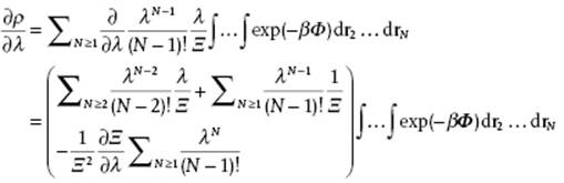
so that

where for the last step the definition g(r₁,r₂) = ρ⁽²⁾(r₁,r₂)/ρ⁽¹⁾(r₁)ρ⁽²⁾(r₂) = ρ⁽²⁾(r₁,r₂)/ρ² is used. Combining the expressions for ∂lnΞ/∂λ and ∂ρ/∂λ yields

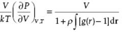
The isothermal compressibility is then given by

Note that the structure factor S(s) for s = 0 reduces to

and therefore S(0) = ρkTκ_T, a fact that can be used for reconstructing g(r).

One might wonder whether the compressibility equation and the pressure equation yield the same result for the pressure. On integrating Eq. (6.40), one obtains

(6.41)

to be compared with P_P as obtained from Eq. (6.39). For the ideal gas g(r) = 1, leading for both expressions to the ideal gas EoS P = ρkT. This is no longer true for a nonideal fluid for which ϕ(r) ≠ 0, and thus g(r) is unknown. Using approximations for g(r) usually leads to different values for P_P and P_κ, indicating a loss of thermodynamic consistency (see Section 6.3).

In order to obtain a complete description of the thermodynamic state, some extra information is required. This is probably most clear from the Gibbs equation

(6.42)

which shows that information is required about the energy U, the pressure P, and the chemical potential μ to obtain a complete description of the thermodynamic state of the system.

If the correlation function g(r) were to be known over a wide temperature range, we could use the energy Eq. (6.32) and integrate the Gibbs–Helmholtz equation and so obtain the required information, since the chemical potential μ can be calculated from the Helmholtz energy F. Similarly, if g(r) were to be known over a wide density range, we could use the pressure Eq. (6.39) and integrate ∂(F/N)/∂(1/ρ) = ρ²P (as obtained from dF = −PdV − SdT + μdN). Alas, neither the temperature nor density dependence of g(r) is usually available.

As an alternative we introduce the coupling parameter approach, also known as thermodynamic integration. A coupling parameter ξ is defined, varying from 0 to 1, which controls the interaction between the reference molecule 1 and another, say j, by replacing ϕ_1j by ξϕ_1j. The potential energy then becomes

(6.43)

and a molecule is added to the system when ξ varies from 0 to 1. The partition function Z_N(ρ,T) reads now Z_N(ρ,T,ξ) while the correlation function g(r;ρ,T) becomes g(r;ρ,T,ξ). Because the number of particles N is very large, we can write

(6.44)

From F = −kTlnZ, we obtain −βF = ln Q_N − ln N! − 3N ln Λ, and hence we get

(6.45)

Further, we have Q_N(ξ = 1) = Q_N and Q_N(ξ = 0) = VQ_N−1. Therefore,

(6.46)

(6.47)

Calculating ∂Q_N(ξ)/∂ξ using Eq. (6.43) results in

(6.48)

Further, employing ρ^(N)(ξ) = N!n^(N)(ξ) with n^(N)(ξ) = Q_N(ξ)⁻¹exp[−βΦ(ξ)], and recognizing that we have N − 1 identical integrals, we obtain

(6.49)

where in the last step ρ⁽²⁾(ξ) = ρ²g(ξ) is employed. Substitution in Eq. (6.45) yields the required result

(6.50)

From , P and μ, we can calculate all of the thermodynamic properties if g(r;ξ) is known. The theoretical calculation of g(r;ξ) is the topic of Chapter 7.

Problem 6.7*

Check the steps necessary to obtain Eqs (6.39), (6.40), and (6.50).