Liquid-State Physical Chemistry: Fundamentals, Modeling, and Applications (2013)

12.6. Structure and Thermodynamics

From the discussion on correlation functions in Section 6.2 we recall that the probability of finding two molecules at distance r is given by n²g(r) with g(r) the (pair) correlation function and n = N/V the number density of N particles in a volume V (note that in Section 6.2 we used ρ = N/V). For independent particles, that probability is given by n². If it is given that the reference molecule is at the origin, the probability of finding a molecule at distance r from the origin is thus ng(r).

12.6.1 The Correlation Function and Screening

These concepts are applied here for ions in solution. We have disregarded the solvent (except for its permittivity) and consider only the correlation between the ions in solution. In the expression for the concentration of counterions iin the neighborhood of a central ion j, Eq. (12.30), we used n_ig_ij(r) with the correlation function for the ions given by

(12.54)

Using Eq. (12.38) we obtain, with B_j given by Eq. (12.37),

(12.55)

As expected, this expression is symmetric in z_i and z_j. Expanding g_ij we obtain

(12.56)

The original Debye–Hückel approximation is given by the first two terms. It might be thought that keeping higher-order terms (or the exponential itself for that matter) is inconsistent with the Debye–Hückel approximation, since in the approximation of Eq. (12.33) the Debye–Hückel approach is self-consistent and obeys the superposition principle for potentials of electrostatics. Pitzer [20], however, has pointed out that for the charged hard-sphere the exponential expression represents the pair-correlation function well, as judged by comparison with Monte Carlo simulations for the same model (Figure 12.6).

Figure 12.6 The pair correlation function at 25 °C for (a) a 0.009 11 M and (b) a 0.425 M aqueous solution of a 1–1 electrolyte with a common hard core value of a = 0.425 nm. The points represent the Monte Carlo simulations, while the solid curve is the exponential Debye–Hückel expression. The dotted and dashed curves are three-term and two-term expansions of the exponential expression, respectively.

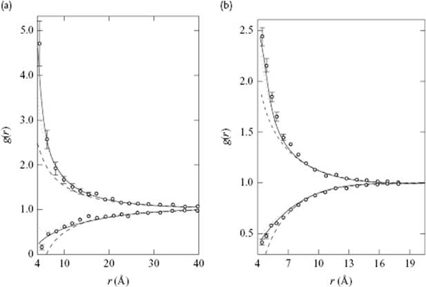
The work done by the system by the charging process leads to a lower potential energy as a result of the approaching of positive and negative charge to approximately a distance of κ⁻¹. In fact, κ⁻¹ is the maximum in the charge distribution 4πr²g_ij(r), so that κ⁻¹ is the most probable thickness of the ionic atmosphere. For a 1–1 electrolyte in H₂O at 25 °C we obtain κ⁻¹ = 3.04 × 10⁻¹⁰ c^−1/2 with c in mol l⁻¹. So, for c = 0.01 mol l⁻¹, the Debye length κ⁻¹ ≅ 3.0 nm. Another interpretation is that for a distance κ⁻¹ the correlation between the ions is largely lost. Because of the formation of the oppositely charged atmosphere of thickness κ⁻¹, the long-range Coulomb potential is screened; this is why κ⁻¹ is also called the Debye screening length.

From the fact that we neglected the structure of the solvent altogether, except for its permittivity, one might guess that the attempts to describe electrolyte liquids by virial expansion would be useful, and this indeed is the case. However, because is of long range, the various integrals for the virial coefficients diverge. McMillan and Mayer showed that, by a clever combination of various expressions, a finite answer can be obtained, and today various advanced theories of ionic solutions employ the virial approach to model the properties of ionic solutions (see, e.g., Friedman (1962) or Barthel (1998)).

Another obvious starting point is to use one of the various integral equations, as they are rather successful in describing liquids, corresponding to highly concentrated solutions. Other approaches, such as the use of perturbation methods, are also available, and for these reference should be made to the specialized literature.

12.6.2 Thermodynamic Potentials*

From all of the above information, the Helmholtz and Gibbs energies of ionic solutions can be calculated. To obtain the required result we integrate with q_j = ez_j. Recall that all are functions of all valencies z_j (see Eq. 12.39). The most convenient way to integrate is to increase the charges of all ions in the same ratio. If we then denote by λ the fraction of their final charges which the ions have at any stage during integration, we have

(12.57)

Using Eq. (12.37) we obtain

(12.58)

(12.59)

From Eq. (12.58) all thermodynamic properties can be calculated in the usual way.

Problem 12.15

Show that the activity coefficient for the solvent is

Problem 12.16*

To show once more the consistency of the Debye–Hückel expressions, derive the activity coefficient for the solute, Eq. (12.42), from G_ele.