Liquid-State Physical Chemistry: Fundamentals, Modeling, and Applications (2013)

12.7. Conductivity

In 1833/1834, Faraday published his law of electrolysis which, in modern terms, states that if two electrodes with a potential difference V are placed in an ionic solution, then material at the electrodes will be liberated, the amount of which is proportional to the amount of charge Q = ∫I dt, where I is the electric current and t the time. Moreover, for a given amount of charge, two elements deposit an amount of material proportional to the equivalent mass, that is, M/z where M is the molar mass and z the charge of the ion. The macroscopic measure of charge F = eN_A is nowadays called the Faraday constant where, as usual, e denotes the unit charge and N_A is Avogadro's constant. Electrolysis can only take place because ionic solutions conduct electricity. The resistance R in Ohm's law R = V/I of a solution in a container of cross-section A and length L is given by

(12.60)

where ρ is the resistivity. One often uses the reciprocal κ = ρ⁻¹, which is addressed as the conductivity⁹⁾. The latter is usually measured in a parallel plate set-up, that is, using a homogeneous system, so that we can also write κ = i/Ewith i = I/A the current density and E = V/L the electric field strength¹⁰⁾. In order to avoid electrode reactions, changing the concentration of the electrolyte in the neighborhood of the electrode, and because the electrolysis products provide an opposing potential (an effect often addressed as polarization), one measures with an alternating potential difference, typically with a frequency in the order of kilohertz. For pure water at 25 °C, κ ≅ 5.5 × 10⁻¹⁰ Ω⁻¹ m⁻¹. For solutions, it is convenient to define the molar conductivity Λ_m = κ/c, where c is the concentration and the equivalent conductivity Λ = Λ_m/n_equ, where the equivalent n_equ = ν₊z₊ = ν₋|z₋| represents the amount of charges released .

Experimental examination of the conductivity revealed that there are two types of ionic solution, as illustrated in Figure 12.7. One type , known as a strong electrolytic solution, has a high and (almost) constant value of Λ that slowly decreases with increasing concentration; examples are NaCl or LiCl in H₂O. An empirical relationship to describe Λ given by Kohlrausch in 1885 [36] is

(12.61)

Figure 12.7 Molar conductivities of CH₃COOH (♦) and NaCl (■) as a function of concentration at 298 K.

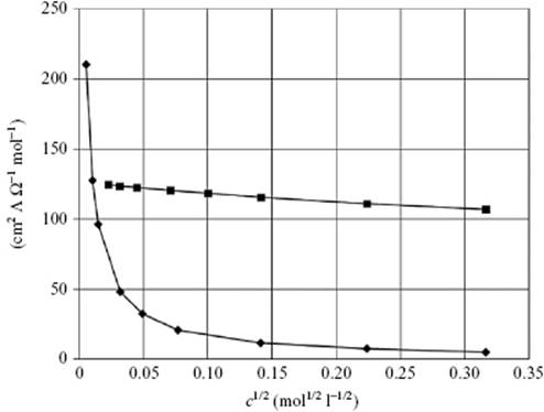
It appears that all 1 : 1 electrolytes have approximately the same value for A.

The other type of ionic solution, known as a weak electrolytic solution, has a much smaller value of Λ which greatly increases with dilution; examples are CH₃COOH and CuSO₄ in H₂O. It should be noted that the labels “strong” and “weak” refer to the combination of solute and solvent. Strong electrolytes in H₂O (e.g., KBr) may be weak in other solvents (e.g., acetic acid). There are relatively few intermediate cases between strong and weak electrolytes. In both cases the limiting value of Λ for c → 0, the limiting conductivity Λ°, plays an important role in theory.

Although it would be beneficial to know the contributions of the individual ions to Λ, it is impossible to determine these contributions from Λ° values alone. Earlier, in 1875, Kohlrausch [37] had noted that the differences in Λ° for pairs of salts having a common ion are approximately independent of that ion. He attributed this effect to independent and additive contributions of the positive and negative ions to Λ°, that is, , usually referred to as the law of independent migration of ions. So, if the single ion conductivity for a particular ion j is known, the rest can be determined.

To obtain these data we consider the speed of ions. The drift speed of an ion s_± is proportional to the electric field E with, as the proportionality constant, the mobility u_±. Suppose that we have a container with field E containing an electrolyte of concentration c. For a salt Q = M_ν+X_ν− dissociating into ν₊M^z+ and ν₋X^z− ions, the concentration of ion j is c_j = ν_jc. The drift speed is then (for positive ions) s₊ = u₊E, and all ions within distance u₊E of the negative electrode will reach that electrode in unit time. The number of such ions is ν₊cu₊E, and these carry a charge z₊Fν₊cu₊E = n_equFcu₊E. Hence, the conductivity κ₊ due to the positive ions is

(12.62)

We further introduce the transport number, t , which reflects the relative contribution of positive and negative charge carriers, that is, not necessarily the molecules or ions as such, to the total current density i and which reads

(12.63)

Since electroneutrality requires ν₊z₊ + ν₋z₋ = 0, the expression for t₊ for a binary electrolyte reduces to

(12.64)

If t₊ can be measured over a range of concentrations, it is possible to extrapolate their values to zero concentration and thus calculate . Note that for weak electrolytes the degree of dissociation α is involved in the total conductivity Λ since c₊ = αν₊c, but not in the transport numbers.

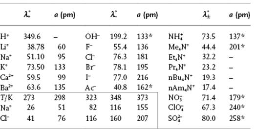
Transport numbers were first measured in 1853 by Johann Wilhelm Hittorf (1824–1914), using an ingenious set-up as sketched in Figure 12.8. In this set-up the amounts of material deposited in the cathode and anode compartments are determined. From the amount of charge and material deposited after a certain time, the number of ions transported can be calculated, leading directly to the transport numbers. It should be noted that during the measurement the concentration changes yielding the result an effective transport number over the changing concentration range during the experiment. Another method for determining the transport numbers is the moving boundary method, which is based on the motion of the interface between two layered electrolyte solutions, visible by differences in either color or refractive index, as a function of the amount of charge passing through the system. Another method which involves measurement of the electromotive force for two combined cells, in one of which the concentration is varied, is also used. We refrain from further details here and refer to the literature [21]. Table 12.8 provides some experimental data from which it can be observed that for increasing ionic radius a, the (equivalent) conductivity λ° also increases, contrary to the expected decrease with ionic radius. This is due to the fact that not the bare but rather the hydrated ion moves. As Δ_hydG decreases with increasing ionic radius, the effective radius decreases. The data for NaCl indicate a strong increase with temperature, and with increasing temperature the average hydration number will decrease so that the effective size becomes smaller, leading to an increase in λ°.

Figure 12.8 Hittorf set-up for measuring ionic velocities. In this case, the ratio of the mobilities of the ions, as determined from the concentrations of the ions in the anode and cathode department, is 1 to 3. Hence, t⁻/t⁺ = 1/3 or t⁻ = t/4 and t⁺ = 3t/4.

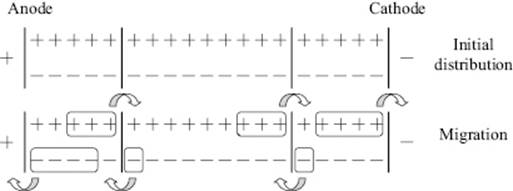
Table 12.8 Limiting ionic conductivities /Ω⁻¹ mol⁻¹ cm² in water at 298 K and for NaCl at various other temperatures. Data mainly from Ref. [19]. The parameter a is the (Pauling) ionic radius or the Kapustinski radius [35], if labeled with an asterisk.

For weak electrolytes, which are typically of 1–1 type, we derived Eq. (12.23), K = α²m/(1 − α), assuming that the activity coefficient γ = 1. Normally, α = Λ/Λ_equ is used as a measure of dissociation, where Λ_equ is the sum of the molar conductivities of the positive and negative ions at the ionic concentration at equilibrium. As the mobility is concentration-dependent, but the ionic concentrations at equilibrium are only known if α is known, an iterative procedure should be used to obtain α. Data obtained in this way, although reasonably constant, show a definite concentration dependence which is the result of neglecting the activity coefficients. By plotting the lnK values obtained versus square-root concentration (αc)^1/2 for a series of diluted solutions, one can extrapolate to zero concentration to obtain the thermodynamic equilibrium constant.

Note from Table 12.8 that the values of λ° for the H⁺ and OH⁻ ions are much larger than for most other ions. Moreover, while hydration data suggest λ°(H⁺) < λ°(Li⁺), in reality λ°(H⁺) >> λ°(Li⁺). In fact, it is the network structure of water and not the hydration shell that determines the anomalous conductance¹¹⁾ of the H⁺ and OH⁻ ions, as explained by the Grotthuss mechanism [22], sketched in Figure 12.9. The protons can easily “debond” from one H₂O to “bond” again to the neighboring H₂O molecule (tunneling), as the hydrogen bonding makes the two configurations already much more similar as otherwise would be the case. It is noteworthy that this process, although faster than translational diffusion, proves to be slower than might be expected from its mechanism. This relative sluggishness may be due to the rotation of molecules required for trains of sequential proton movement and the consequential necessity for the breakage of hydrogen bonds. The strange effect [23] of degassing increasing proton motion over tenfold indicates, however, that nonpolar dissolved gas molecules (which are naturally present) disrupt the linear chains of water molecules necessary for the Grotthuss mechanism and so slow down the proton movement. Other mechanisms have also been proposed.

Figure 12.9 Schematic of the Grotthuss mechanism.

Although, in the past, a mechanism similar to that for the H⁺ ion was assumed to operate for the OH⁻ ion, today it is thought that the movement of the OH⁻ ion is accompanied by a fourth hydrogen-bonded donor water molecule. The hydrated hydroxide ion is coordinated to four electron-accepting water molecules such that when an incoming electron-donating hydrogen bond forms (necessitating the breakage of one of the original hydrogen bonds) a fully tetrahedrally coordinated water molecule may be easily formed by hydrogen ion transfer.

12.7.1 Mobility and Diffusion

The mobility as determined from electrical conductivity is related to the diffusivity, and this can be seen as follows. The driving force for diffusion is given F_dri = −(kT/c)dc/dx (ignoring the difference between activity a and concentration c), while the frictional force is proportional to the drift speed s, that is, F_fri = fs, where f is a friction coefficient and 1/f a mobility coefficient. Under steady-state conditions these two forces are equal and so fs = −(kT/c)dc/dx. Defining the flux j by j ≡ cs we obtain

(12.65)

Comparing this expression with Fick's first law, j = −D(dc/dx), we obtain the equation, first derived in 1905 by Albert Einstein (1879–1955),

(12.66)

where the last step can be made if the frictional force is given by Stokes' law F_fri = 6πηas, where η is the viscosity and a is the radius of the charge carrier (ion plus hydration shell). In this form it is referred to as the Stokes–Einstein equation. In the electric case the driving force F_dri for a positive ion with charge z₊e in an electric field E is given by F_dri = z₊eE, while its frictional force F_fri is proportional to its speed, F_fri = f₊s₊. Under steady-state conditions the forces F_dri and F_fri are equal and opposite, and thus z₊eE = f₊s₊. Because the speed is also given by s₊ = u₊E, where u₊ is the mobility, we obtain f₊ = z₊e/u₊. Inserting this result into Eq. (12.66) leads to the Einstein equation

(12.67)

Writing , we can also write , known as the Nernst–Einstein equation, first derived in 1888 by Walther Nernst (1864–1941). A similar equation can be written down for D₋. To obtain the diffusion coefficient for ambipolar diffusion of a symmetrical electrolyte in a solution, the diffusion coefficients of the positive ions D₊ and negative ions D₋ must be combined via

(12.68)

Problem 12.17: Conductivity of water

Make an estimate of the lifetime t_H of hydrogen bonds in water from its ionic conductance, based on the Grotthuss mechanism.

Problem 12.18: Ionic conductivity

Consider a Teflon tube with Pt electrodes that close the ends of the tube (tube cross-section 5 cm², tube length 10 cm). The tube is filled with an aqueous solution of 0.01 M CaI₂ and a voltage of 10 V is set across the tube.

a) Calculate the rise in temperature ΔT for preparing this solution.

b) What is the molar conductivity Λ_m of CaI₂?

c) Calculate the electrical current I on the basis of data.

d) Calculate I using for the ions the Stokes–Einstein equation F = 6πηas (F friction force, η viscosity, a radius and s velocity) and the Pauling ionic radii, and compare the result with that obtained in (c).

e) What is the transport number t of Ca²⁺ in this case?

f) Suppose that the tube and electrodes have a negligible thermal capacity and are thermally perfectly isolated from the surroundings. What is the temperature rise per second of the solution in the tube, given that C_P(solution) ≅ 4180 J kg⁻¹ K⁻¹?

Problem 12.19: Diffusion coefficient*

Derive Eq. (12.68) for electrolyte Q = M_ν+X_ν− using a 1D configuration. Do so by equating the flux of the positive and negative ions in terms of the electrochemical potential and solving this equation for dϕ/dx. Note that the electrochemical potential for component α is defined as , and that in equilibrium for every point in the solution. By substituting dϕ/dx in , calculate the flux j_Q and identify the proportionality constant as the diffusion constant D.