Liquid-State Physical Chemistry: Fundamentals, Modeling, and Applications (2013)
12. Mixing Liquids: Ionic Solutions
12.8. Conductivity Continued*
Let us continue with conductivity and try to explain the Kohlrausch expression Eq. (12.61). One can ask two questions with respect to this equation: why is the dependence c1/2; and what is the value of the constants Λ° and A. To explain this we must consider that when an ion in solution is dragged through the solution by an applied electric field, two extra effects are present. The first is the electrophoretic effect, and the second is the relaxation effect. Thereafter, we discuss ion association.
Let us consider first the electrophoretic effect, first described by Onsager and Fuoss in 1932. The total net charge of an ion atmosphere is equal and opposite to that of the central ion. If, therefore, under the influence of an applied electric field, the central ion moves to the right (positive direction) the atmosphere will move to the left (negative direction). The central ion therefore finds itself in a stream of solution moving opposite to the direction of the central ion, diminishing its net velocity. If the ionic strength becomes smaller, the atmosphere becomes more extended and the effect smaller.
Since bulk flow of the solution is negligible, it follows that the force fj acting on ion j must be balanced by the force fs acting on the solvent molecules, and thus we have Σjnjfj + nsfs = 0, where the number density is given by nj. The local density of ions i around a central ion j in a volume element dV reads nij = nigij(r), determined by the distribution function gij(r) as given by Eq. (12.56). Therefore, the force near ion j will be Σinijfi dV which is different from the volume-averaged force ΣinifidV. Since the solvent is neutral, the local density is the average density and the force on the solvent is given by nsfsdV = −Σinifi dV. The net force dFj acting on ion j is therefore
(12.69) ![]()
where the last step can be made if we take for dV a spherical volume element with radius r and thickness dr. Evaluating the dFj on this volume element by approximating gij by Eq. (12.56), the result becomes
(12.70) ![]()
(12.71) ![]()
This force is counteracted by the friction experienced by ion j and its atmosphere, as described by Stokes' law. So, for the drift speed change we have Δsj = dFj/6πηr, where η is the viscosity of the medium and r the radius of each volume element. This leads to
(12.72) ![]()
Let us now turn our attention to the relaxation effect, already considered by Debye and Hückel in 1923, but more successfully by Onsager in 1927 and extended in 1954 by Falkenhagen [21]. The basic idea is that there will be a disturbance of the spherical symmetry of the atmosphere if the central ion moves under the influence of the applied field. If, for example, a specific type of ion moves to the right, each ion will constantly have to build up its ionic atmosphere to the right, while the charge density to the left gradually decays. The rate at which this occurs is related to the relaxation time τ of the atmosphere. The time required for the atmosphere to fall essentially to zero is 4hτ, where
(12.73) ![]()
and where z and λ have the same meaning as before. The relaxation time appears to be
(12.74) ![]()
where f is the friction force constant for a single ion. Due to this finite relaxation time, the atmosphere will lag behind the moving central ion by approximately τ scen and deviate from the spherical symmetry. As a consequence, there will a backwards pull on the central ion, which for a solvent with permittivity ε has been calculated by Onsager and Falkenhagen et al. as
(12.75) ![]()
where ΔE is the relaxation electric field acting in the opposite direction of E and the constant H ≡ h/(1 + h1/2) is introduced. Adding the field of the relaxation effect to the applied field leads to the total force fj on an ion j given by
(12.76) ![]()
The force fj produces a velocity ![]() relative to the solvent that becomes
relative to the solvent that becomes
(12.77) ![]()
with ![]() the limiting mobility, as defined by the limiting velocity at infinite dilution
the limiting mobility, as defined by the limiting velocity at infinite dilution ![]() . The force fj is also the force that has to be used in Eq. (12.71) for evaluating the electrophoretic velocity drag Δsj. Evaluating Δsj with this force leads to
. The force fj is also the force that has to be used in Eq. (12.71) for evaluating the electrophoretic velocity drag Δsj. Evaluating Δsj with this force leads to
(12.78) ![]()
where ![]() is the exponential integral and where
is the exponential integral and where ![]() , Eq. (12.33), is used. For symmetrical electrolytes z1 = −z2 and, since fi in Eq. (12.71) is proportional to ezi, A2 will vanish.
, Eq. (12.33), is used. For symmetrical electrolytes z1 = −z2 and, since fi in Eq. (12.71) is proportional to ezi, A2 will vanish.
Although we have included the second-order electrophoretic term, we recall that a mathematically consistent solution of the Poisson equation in combination with the Boltzmann distribution can be taken only as far as first order for unsymmetrical electrolytes and to a second-order term for symmetrical electrolytes. However, since for symmetrical electrolytes the second-order term with A2 vanishes anyway, we need to consider only the first-order term. The final drift speed (to first order) then becomes
(12.79) ![]()
The ratio ![]() , and the conductivity λj of ion j becomes
, and the conductivity λj of ion j becomes
(12.80) ![]()
using ![]() with F the Faraday constant. Combining the expressions for the positive and negative ions in the usual way via Λ = λ+ + λ−, introducing
with F the Faraday constant. Combining the expressions for the positive and negative ions in the usual way via Λ = λ+ + λ−, introducing ![]() , Eq. (12.48), and neglecting cross terms results in the equivalent conductivity, we obtain
, Eq. (12.48), and neglecting cross terms results in the equivalent conductivity, we obtain
(12.81) ![]()
Here, S is a complex constant, dependent on temperature, charge and (limiting) conductivity of the ions and relative permittivity and viscosity of the solvent, given by
(12.82) ![]()
For a symmetrical electrolyte we have z1 = z2 = z. The relevant data for water at 25 °C are: εr = 78.30 and η = 0.8903 mPa s. Expressing the value for Λ in cm2 Ω−1 mol−1, the values of P and Q reduce to
(12.83) ![]()
This model explains why the conductivity of strong electrolytes is described to first order by Λ = Λ° − Ac1/2 and provides a value12) for A. Moreover, it gives a fair account of the conductivity of aqueous solutions of 1–1 electrolytes up to 0.05 or 0.1 m. For other electrolytes the situation is less favorable. Robinson and Stokes [21] showed that the convergence of the model using the full expansion of Eq. (12.54) depends mainly on the factor ![]() , where n is the order of the expansion. Because most ions have a radius of, say, 4 Å, it will be clear that convergence for 1–1 electrolytes is reasonable and the behavior can be described by the truncated expression Eq. (12.56). Although for 2–2 electrolytes the second-order term vanishes, the third-order term is about as large as the first- order term, and hence a more extensive theory is called for. Also, for higher concentrations a more extensive theory is required. These theories are beyond the scope of this book.
, where n is the order of the expansion. Because most ions have a radius of, say, 4 Å, it will be clear that convergence for 1–1 electrolytes is reasonable and the behavior can be described by the truncated expression Eq. (12.56). Although for 2–2 electrolytes the second-order term vanishes, the third-order term is about as large as the first- order term, and hence a more extensive theory is called for. Also, for higher concentrations a more extensive theory is required. These theories are beyond the scope of this book.
12.8.1 Association
A regularly occurring deviation in plots of Λ versus c1/2 is that the (negative) slopes are larger than predicted by the Debye–Hückel–Onsager model, which means that the experimental conductivities are smaller than predicted. Estimating ionic radii from the fitted parameters often yielded unphysically small radii. In essence, there are two ways to remedy the situation. The first approach is to extend the Debye–Hückel–Onsager solution of the Poisson–Boltzmann equation to a higher order (a brief discussion can found in Fowler and Guggenheim [24]), but this solution does not have the property of self-consistency, in contrast to the first-order solution. This implies, for example, that if the activity is calculated from the electrostatic energy (see Problem 12.15), the result deviates from the result as obtained via the Güntelberg procedure (see Section 12.5). Here, we address the alternative, second approach that takes ion association into account.
Recall that in the Debye–Hückel–Onsager model, the complete dissociation of ion pairs is assumed. This is not necessarily true, however, and in 1926 Niels Bjerrum [25] introduced a theory in which ions of opposite charge would temporarily form an associated pair via Coulomb forces. A reference ion, say a positive ion at the origin, and a counterion, say a negative ion at distance R, are considered to be an ion pair if no other ions can be found in the sphere with radius R centered at the reference ion. For ease of presentation, we limit the discussion to symmetric ionic solutions (z1 = z2), so that an ion pair (IP) in solution is neutral. We denote the ionic radii by a1 and a2. It appears to be convenient for later to introduce the parameter q = z1z2e2/8πεkT, nowadays called the Bjerrum length.
We first need to discuss the expression for the energy difference W between two (solvated) ions and the ion pair. To zeroth order this is given by the Coulomb expression WC(r) = e2z1z2/4πεr. However, from the Debye–Hückel theory we know that in an ionic solution shielding of the Coulomb potential occurs and Eq. (12.38) applies. However, it should be noted that the shielded Coulomb potential applies only outside the sphere of the bound ion pair as there are no other ions inside the sphere. Moreover, apart from the Coulomb forces, we also have the induction, dispersion, and repulsion forces. Finally, we have also to consider the effect of the solvation shells. Each ion has a solvation shell, and if ions come close together these shells interpenetrate and this leads to an interaction force, often termed the Gurney force. Hence, these interactions together can be represented as the sum of the Coulomb interaction WC(r) and a short-range part WSR(r), the latter being the sum of the induction, dispersion, Gurney, and repulsion forces. A simple but effective representation of WSR(r) is given by
(12.84) 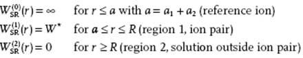
Now, the Debye–Hückel model has to be solved for the potential W = WC(r) + WSR(r) in the three regions indicated. Similar to the original Debye–Hückel model, the potential as well as its derivative must be continuous at r = R(as well as r = a). This leads for region 2 right away, in the same way as in Section 12.5, to
(12.85) ![]()
For region 1, no ions are present between the reference ion and the counterion. In principle, the Coulomb potentials WC(r) = z1z2e2/4πεr = 2qkT/r acts, but since the potential and derivative should match with ![]() at r = R, the potential is modified to
at r = R, the potential is modified to
(12.86) ![]()
Now, we are ready to deal with association reaction. In Chapter 6 we learned that the number of molecules in a sphere with radius R is given by the integral over the radial distribution function g(r). We apply the same expression here, but modified for an ionic solution with concentration of ions c and degree of dissociation α. Approximating g(r) by ![]() with β = 1/kT, the number N of dissociated ions in a sphere of radius R is given by
with β = 1/kT, the number N of dissociated ions in a sphere of radius R is given by
(12.87) ![]()
The lower limit of the integral is taken as a = a+ + a−, since this is the distance of closest approach. Inserting Eq. (12.86) the result becomes
(12.88) ![]()
For the association reaction ![]() in the sphere we have
in the sphere we have
(12.89) ![]()
The fraction bound ion pairs with respect to the number of ions is thus (1 − α)/α. Since the actual number of ions in the sphere is given by N, we obtain
(12.90) ![]()
Now consider the association constant ![]() of the reaction in terms of activities. Let us assume that the activity coefficient of the bound ion pair γIP = 1. For the ions, the activity coefficient
of the reaction in terms of activities. Let us assume that the activity coefficient of the bound ion pair γIP = 1. For the ions, the activity coefficient ![]() as given by Eq. (12.45), but with the distance of closest approach a replaced by R. In that case,
as given by Eq. (12.45), but with the distance of closest approach a replaced by R. In that case, ![]() is given by
is given by
(12.91) ![]()
with Kass the association constant in terms of concentrations. Using Eq. (12.88) and (12.90), combined with the expression for ![]() , we find
, we find
(12.92) ![]()
The activity coefficient with respect to the total amount of ions dissolved becomes ![]() . Since the final set of expressions is coupled, an iterative solution is required.
. Since the final set of expressions is coupled, an iterative solution is required.
However, before solving the equations, a choice for R and W* must be made. It appears that with increasing distance r from the reference ion, there is a decreasing probability of finding a counterion per unit volume. The volume of the shell increases, however, and these effects when combined yield a minimum probability of finding a counterion on the sphere around the reference ion for R = q.
So, Bjerrum [25] selected R = q and ignored W*, while much later – taking a somewhat different point of view – Fuoss [26] chose R = 4a/3 and W* = 0. Fuoss [27] also presented a more elaborate theory which showed that the precise choice of R is immaterial since by using a value of ½q or 2q instead of q, the result would differ only insignificantly. For water at 25 °C with εr = 78.3, one calculates for z1 = z2 = 1, q = e2/8πεkT = 0.358 nm, and at this distance the electrostatic energy is 2kT. This energy, being fourfold the kinetic energy, is sufficient to have a significant ion association, albeit of a dynamic nature with rapid exchange with the surrounding ions. Hence, we can say that if ions are closer than 0.358 nm, they are associated. For multivalent ions with charge ez, q = |z1z2|e2/8πεkT, implying that in water association occurs at a distance |z1z2|·0.358 nm. While for univalent ions it is difficult to approach each other closer than 0.358 nm and associate, the q expression for ions of higher charge shows that, for these ions, association is much more important. From the above it also follows that ion association is much more important for solvents with a low relative permittivity.
There remains only a discussion of the agreement with experiment, which we limit here to just two examples. Bjerrum [25] showed that values for the distance of closest approach a, as calculated from the osmotic coefficient g, yielded much more reasonable values than with the Debye–Hückel–Onsager theory, especially for bivalent ions as well as for univalent ions in low permittivity solution, such as alcohols. A decisive set of experiments on the conductivity of solutions of tetra-iso-ammonium nitrate in mixtures of water and dioxane, covering a wide range of relative permittivities from 2.9 to 78, was presented by Fuoss and Krauss [28]. On applying the Debye–Hückel–Onsager model, marked deviations for the limiting conductivity from experiment were observed for low-permittivity solutions. Using Bjerrum's equations it appeared that, assuming a distance of closest approach of ∼0.64 nm , Kasswas indeed constant over the range of εr used. This is a severe test in view of the range of εr used.