Liquid-State Physical Chemistry: Fundamentals, Modeling, and Applications (2013)
13. Mixing Liquids: Polymeric Solutions
13.5. EoS Theories*
In the FH approach it is assumed that the Helmholtz energy F is fully determined by the temperature (and composition), and that volume is not an explicit variable. In reality, the volume does change, and this leads to Equation of State (EoS) theories in which both temperature and volume are taken explicitly into account. In this section, we outline a few of these theories in which use will be made of various aspects of lattices and holes, as discussed in Chapter 8. When using a lattice theory, one has three options to include “free volume”:
· The first option is to use temperature-dependent cell volumes, which is addressed as cell theory.
· The second option is to introduce empty cells or holes (while keeping the cell volume constant); in Chapter 8 for simple and normal liquids this was referred to as hole theory, but in relation to polymer solutions it is often termed the lattice fluid (or lattice gas) theory.
· The third option is to combine these approaches, in relation with polymers often denoted as hole theory, in obvious contradiction to the terminology as used for simple fluids.
An example of each of these options is discussed below, but first we briefly review basic cell theory and its extension to chain molecules.
13.5.1 A Simple Cell Model
In Section 8.2, we learned that for the cell model with N molecules in a volume V on a lattice with coordination number z, using a Lennard-Jones potential with hard-core parameter σ, or alternatively an equilibrium distance r0 = 21/6σ, an energy well depth ε, and expanding the lattice from σ to a to mimic free volume for the liquid, the configurational partition function Q is given by
(13.73) ![]()
where E0 = ½zNϕ(0) represents the lattice energy of the cell model and ϕ(0) represents the pair energy for all molecules (segments) occupying the origin of their cell. In connection with polymer mixtures, this quantity is sometimes referred to as contact energy. Using v0 = V0/N ≡ γ−1σ3 = γ−1(2−1/6r0)3 or6) ![]() and va = V/N ≡ γ−1a3 with γ = 21/2 for a FCC lattice, ϕ(0) is given by
and va = V/N ≡ γ−1a3 with γ = 21/2 for a FCC lattice, ϕ(0) is given by
(13.74) ![]()
Here, A = 1 and B = 1 if one includes only nearest-neighbor interactions, and A = 1.011 and B = 1.2045 using the lattice sum for the FCC lattice. If we have for the total potential ϕ(r) = ϕ(0) + ψ(r) with ψ(r) the vibrational part, the free volume is given by
(13.75) ![]()
Approximating the potential ψ(r) by a square well with radius (a − σ), the free volume vf becomes
(13.76) ![]()
For the configurational Helmholtz energy Fcon = −kTlnQ, we thus have
(13.77) ![]()
Because P = −∂F/∂V and in F = Fkin + Fcon ≡ −kT lnΛ−3N − kT ln[Q(1)N], with as usual Λ = (h2/2πmkT)1/2, only Fcon depends on V, we have
(13.78) ![]()
Introducing the reduced variables v = va/v* (with ![]() ), t = T/T* where T* = zε/k and p = P/P* where P* = zε/v* = kT*/v*), this expression becomes
), t = T/T* where T* = zε/k and p = P/P* where P* = zε/v* = kT*/v*), this expression becomes
(13.79) ![]()
For a small molecule, the external degrees of freedom (DoF) – that is, translation and rotation – are fully available. However, for a chain each of the r segments of the N polymer molecules cannot move completely freely because they are bonded covalently to their neighbors. Prigogine et al. [14] solved this issue empirically by proposing that only a fraction c of the external DoF, in particular the “lower” frequency modes that are available for “completely free segments,” are available as external DoF for chain-like molecules. By accepting this, the exponent 3 in the expression for vf changes to 3c, and the volume v = V/rN now refers to the segment volume. The lattice energy does not change, except that the coordination number might be altered. Hence, instead of Eq. (13.77) we have
(13.80) ![]()
The reduced EoS remains the same but with reduced variables v = va/v* (with ![]() ), t = T/T* where T* = zε/ck and p = P/P* where P* = zε/v* = ckT*/v*). In total, we thus have three parameters: zε, v*, and c (or alternatively, P*, v*, and T*).
), t = T/T* where T* = zε/ck and p = P/P* where P* = zε/v* = ckT*/v*). In total, we thus have three parameters: zε, v*, and c (or alternatively, P*, v*, and T*).
On extending this simple cell (SC) model to solutions, one assumes that the EoS expression obtained for the pure liquid is also valid for solutions. Since this model has three parameters, in order to describe solutions one also requires three combining rules. It appears – as might be expected – that a geometric combining rule for ε is not sufficiently accurate, and therefore ε is often determined experimentally, for example, from the heat of mixing. One also needs to take into account various ways in which the molecules can be distributed over the lattice, and this is done by adding, for example, a FH-type entropy term. In general, this leads to an extra combinatorial factor g(Y) in Eq. (13.73), where Y indicates the set of relevant variables. Using a cell model for a pure component g = 1, but for a (binary) solution with Nj molecules of type j, we have the set Y = (N1,N2). For a lattice theory for a pure component of N molecules we have Y = (N,ϕ), with ϕ the volume fraction occupied cells, whereas for a solution we have Y = (N1,N2,ϕ). The latter set also applies to a hole theory.
13.5.2 The FOVE Theory
Apart from contributing to the above-discussed FH theory, Flory also contributed the EoS theories and, together with some collaborators, constructed what presently is known as the Flory–Orwoll–Vrij–Eichinger (FOVE) theory [15]. In this theory, a lattice is again assumed on which the solute segments and solvent molecules are distributed with no additional holes –that is, it is a cell model.
For larger volumes, the attractive part in Eq. (13.74) proportional to v−2 dominates, and Flory et al. argued that, in the spirit of the vdW theory, ϕ(0) should be replaced by ϕ(0) = −sη/v. Here, η is the energy parameter associated with the segment–segment contact (with dimension J m3 instead of J only, as for ε), s is the number of such contacts per segment, and v is the segment volume. Furthermore, Eq. (13.76) is accepted for the free volume so that Fbecomes
(13.81) ![]()
Following the usual route of calculating P = −∂F/∂V, the reduced EoS obtained reads
(13.82) ![]()
The more usual form of the FOVE EoS is obtained by replacing 2−1/6 by 1, resulting from the use of the LJ potential. This does not influence the EoS if the reducing parameters are defined accordingly. The reducing parameters are usually obtained by fitting to data for pure liquids. This model gives a reasonable description for pure polymer liquids, taking reasonable ranges of temperature and pressure.
On changing to solutions, we now need to state how we obtain the combining rules for the reduced variables which we can take to be v*, T* and c, recalling that P* = ckT*/v*. If we use the same segment volume for both components, we obtain from the EoS of the pure polymers ![]() , and therefore
, and therefore ![]() . Hence, we need only two combining rules, either for T* and P* or for c and r. From the energy term for pure liquids in Eq. (13.81), U = −½rNsη/v = rNP*(v*)2/v. Using the same reasoning as for Eq. (8.37), but with possibly different coordination numbers s1 and s2 for components 1 and 2, respectively, we have
. Hence, we need only two combining rules, either for T* and P* or for c and r. From the energy term for pure liquids in Eq. (13.81), U = −½rNsη/v = rNP*(v*)2/v. Using the same reasoning as for Eq. (8.37), but with possibly different coordination numbers s1 and s2 for components 1 and 2, respectively, we have
(13.83) ![]()
We approximate now the number of unlike pairs by N12 = (s1r1N1) (s2r2N2)/srN, where we use r = (r1N1 + r2N2)/N and s = (s1r1N1 + s2r2N2)/rN. The energy of the mixture (in the notation of the present paragraph and using ηinstead of ε) becomes
(13.84) ![]()
where Δη = η11 + η11 − 2η12. The volume fractions for the segments read ϕj = rjNj/rN, and therefore the energy becomes
(13.85) ![]()
Using ![]() for the pure liquids, one easily transforms this expression to
for the pure liquids, one easily transforms this expression to
(13.86) ![]()
Comparing with U = −rNP*(v*)2/v, one obtains
(13.87) ![]()
with ![]() . Writing for the number of external DoF c = (c1r1N1 + c2r2N2)/rN = ϕ1N1 + ϕ2N2, the use of the reduced variables T* = P*v*/ck and
. Writing for the number of external DoF c = (c1r1N1 + c2r2N2)/rN = ϕ1N1 + ϕ2N2, the use of the reduced variables T* = P*v*/ck and ![]() yield
yield
(13.88) ![]()
Finally, the reduced Gibbs energy Gred = G/rNε* (with G = F + PV and ε* = −½zε) reads
(13.89) ![]()
where, obviously, the reduced variables and their combining rules must be used. From this expression all other properties can be calculated in the usual way.
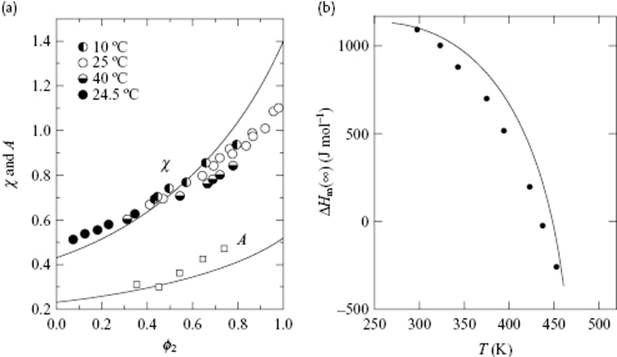
We provide only one example for comparison with experiment. Figure 13.8a shows the apparent χ parameter and its enthalpic part A [Eq. (13.55)] for a solution of polyisobutylene in benzene. Although evidently not perfect the agreement is, nevertheless, quite good.
Figure 13.8 (a) Apparent χ and enthalpic A parameters (Eq. 13.55) versus segment volume fraction ϕ2 for polyisobutylene in benzene as calculated from the FOVE EoS theory. The entropic B parameter is the difference between χand A. The symbols indicate the experimental data points, while the curves are calculated from the FOVE theory; (b) A comparison of experimental (solid circles) and theoretical (solid line) heats of mixing for dilute solutions of polyisobutylene in benzene. The theoretical curve was calculated from the LF EoS theory, using temperature-independent pure-component parameters.
13.5.3 The LF Theory
Sanchez and Lacombe [16] proposed another means of discussing polymer liquids and solutions. In essence, this theory – labeled as the Lattice Fluid Theory (LFT) – is a straightforward extension of the hole theory of molecular solutions to polymer molecules. A fixed cell size of volume v* is chosen, and the overall volume change occurs via the introduction of extra holes. For a polymer solution with r segments for the N molecules, the volume is V = N0 + rN if N0 holes are present. If ϕ = N/(N0 + rN) is the fraction of cells occupied, then we obtain for the energy (similar to Section 8.3), U = ½rNϕzε, where ε refers to the segment–segment interaction. Hence, Eq. (13.54)becomes
(13.90) ![]()
Again, following the usual route of calculating P = −∂F/∂V = −∂F/∂(V/v*) = −∂F/∂N0, the EoS is obtained which in this case reads
(13.91) ![]()
or in reduced form
(13.92) ![]()
with reduced variables v = v*/(V/rN), ρ = 1/v = ϕrNv*/V and t = T/T*, where T* = ε*/k, ε* = −½zε and p = P/P*, with P* = ε*/v* = kT*/v*. Here, we have also three parameters: two reduced parameters, v* and ε* (or alternatively v* and T*) and the DP, r. Again, these parameters are obtained by fitting to data for pure liquids. This model also gives a reasonable description for pure polymer liquids, taking reasonable ranges of temperature and pressure. The reduced Gibbs energy g = G/rNε* with G = F + PV reads
(13.93) ![]()
For solutions, Sanchez and Lacombe estimated the combining rules for v* and r as follows. The first assumption is that the close-packed volume is additive. Denoting the DP for pure components by ![]() , and for the mixture by rj, the volume of the mixture becomes
, and for the mixture by rj, the volume of the mixture becomes ![]() , which implies
, which implies ![]() . Accordingly,
. Accordingly, ![]() , as was also obtained for the FOVE theory. The second assumption is that the number of pair interactions in the mixture is the same as the sum of those interactions in the pure liquids. Hence,
, as was also obtained for the FOVE theory. The second assumption is that the number of pair interactions in the mixture is the same as the sum of those interactions in the pure liquids. Hence, ![]() , where N = N1 + N2. These two assumptions lead to
, where N = N1 + N2. These two assumptions lead to
(13.94) ![]()
where, as usual, xj denotes the mole fraction. This further leads to
(13.95) ![]()
The combining rule for P* follows the FOVE approach, but s1 and s2 are assumed to be equal and thus
(13.96) ![]()
where ![]() now can be taken as a parameter independent of composition since s1 = s2. From these results it follows that ε* = kT* = P*V*. Adding the entropy term, one finally obtains for the reduced Gibbs energy g = G/Nrε*
now can be taken as a parameter independent of composition since s1 = s2. From these results it follows that ε* = kT* = P*V*. Adding the entropy term, one finally obtains for the reduced Gibbs energy g = G/Nrε*
(13.97) ![]()
using the same reduced variables as for Eq. (13.89). From this expression all other properties can be calculated in the usual way.
Also here we provide only one comparison with experiment. Figure 13.8b shows the heats of mixing for dilute solutions of polyisobutylene in benzene with a quite good agreement with experiment.
13.5.4 The SS Theory
Another approach is due to Simha and his collaborators. In particular, Simha and Somcynski [17] (SS) described a pure polymer liquid, which was extended later by Jain and Simha [18] to solutions. This, in polymer solution jargon, is a hole theory. A recent perspective has been provided by Moulinié and Utracki [19].
Employing, as before, for each of the N molecules the equivalent chain with r segments and denoting the fraction occupied cells with ϕ, we have ϕ = rN/(rN + N0). The configurational partition function Q is given by Eq. (13.73), with the additional combinatorial factor g(X) for solutions. In the original SS theory for g(X) the FH-form was chosen which, keeping only the pertinent part, reads g(N,ϕ) = ϕ−N(1 − ϕ)−rN(1−ϕ)/ϕ for pure compounds. Instead of using ½zNϕ(0), one uses the expression ½qczNϕεc, where the number of nearest-neighbor sites per chain qcz = r(z − 2) + 2 replaces the coordination number z, and the introduction of the volume fraction ϕ corrects for the presence of holes. The contact energy for a pair of segments εc replaces ϕ(0), as given by Eq. (13.74) while the volume va = ϕV/rN = ϕv again refers to the average volume per segment. Similarly, as in the Significant Liquid Structures (SLS) theory (see Section 8.4), the free volume is estimated as an average of a solid-like contribution vf,s and a gas-like contribution vf,g, so that
(13.98) ![]()
Finally for the number of external DoF 3c is used so that the partition function Q(N,ϕ), now a function of N and ϕ, reads
(13.99) ![]()
The various properties follow from F(N,ϕ) = −kTlnQ(N,ϕ), where the optimum value for ϕ is obtained from ∂F/∂ϕ = 0, leading to
(13.100) ![]()
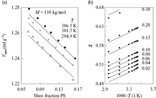
with L(ϕ,v) = [2−1/6ϕ(ϕv)−1/3 − 1/3]/[1 − 2−1/6ϕ(ϕv)−1/3]. As usual, the EoS is obtained from P = −∂F/∂V. Solving the coupled equations, Eq. (13.100) and the pressure equation, leads to the SS description. Taking r = c = q = 1, one obtains the expressions for simple, spherical molecules. The theory was tested on Ar, for which it appeared that the volume of the cell at zero pressure is remarkably constant at about 0.96v* to 0.98v*, while as a function of volume and temperature the volume varied between 1.02 for 1/v = 0.05 and t = 1.20, and 0.84 for 1/v = 0.70 and t = 3.0. The (reduced) critical constants were predicted to be vcri = 3.9 (3.16), tcri = 1.27 (1.26) and pcri = 0.115 (0.116), showing fair agreement with the experimental data (shown in brackets). For chain-like molecules the cell volume depends weakly on the ratio r/3c, so that often a universal value of r/3c = 1 is chosen. Figure 13.9 shows the comparison with experiment for the specific volume for polystyrene–cyclohexane mixtures, showing quite reasonable agreement.
Figure 13.9 (a) Comparison of the specific volume Vspec of polystyrene–cyclohexane mixtures as a function of composition at different temperatures. The points show the experimental data, while the lines represent the result of the SS theory; (b) Comparing the apparent χ parameter for polystyrene (Mw = 520 kg mol−1) in cyclohexane as a function of temperature. The points show the experimental data, while the lines represent the result of the HH theory.
Several extensions for the SS theory have been proposed [20], the first of which is the Holey Huggins (HH) theory.7) Whereas, in the original SS theory the external contact parameter q was evaluated via qcz = r(z − 2) + 2, in the HH theory the refinement is made to take the occupied fraction ϕ into account via q = Nqcz/(Nqcz + zN0) = (1 − α)ϕ/(1 − αϕ), where α = 2(1 − r−1)/z. This leads essentially to the Huggins [4] expression for the entropy. Obviously, for 2/z → ∞, α → 0 and the HH theory reduces to the SS theory.
This modification leads to
(13.101) ![]()
![]()
The Huggins expression for the combinatorial function g is in considerable better agreement with simulation results then the FH-expression.
However, the random nature of the entropy term remains. Using the quasi-chemical approximation, an improvement labeled as non-random mixing (NRM) HH theory results. To that purpose, a parameter X is introduced which takes in to account the fraction of segment–hole contacts. Denoting the total number of contacts by Q = ½z(Nqc + N0) = ½zNqc/q, the product QX is the number of segment–hole contacts, while the number of segment–segment contacts is Q(q − X) and the number of hole–hole-contacts is Q(1 − q − X). The combinatorial function g is now described by Eq. (C.24), while E0 and vf become
(13.102) ![]()
Here, X/q represents the fraction of segment–hole contacts with respect to the total number of external contacts, and 1 − X/q the remaining fraction of segment–segment contacts. As usual, the optimum parameters are determined by minimization with respect to ϕ and X, that is, from ∂F/∂ϕ = 0 and ∂F/∂X = 0. Figure 13.9 shows a comparison of the specific volume of polystyrene–cyclohexane mixtures as function of composition at different temperatures, as well as the apparent χ parameter for polystyrene in cyclohexane as a function of temperature. The agreement is quite fair.
Simplifications for the SS theory have also been proposed. These attempts have been focused on providing an explicit expression for ϕ, so that solving coupled equations becomes unnecessary. A relatively simple approach that, nevertheless, provides results as good as the original SS theory is to replace [21] the expression for ϕ by 1 − ϕ = exp(−c/2st), as inspired by the expression for the fraction of vacancies in a solid. This decouples the original SS equations, Eq. (13.100) and the pressure equation P = −∂F/∂V. Subsequently (for one reason or another), the commonly used FCC lattice with z = 12 was replaced by the BCC lattice with z = 8. The authors refer to this model as the simplified hole theory (SHT). When comparing 67 polymers and 61 solvents, the conclusion was that SHT performed for the polymers as well as the SS theory – that is, there was a grand average deviation D for the density over all compounds and temperature ranges available of D = 0.066 and D = 0.065, respectively. For solvents, the SHT was only slightly worse, with D = 0.097 for the original SS theory and D = 0.125 for SHT. Simha et al. [22] also proposed a simplification by using a fitted expression for the fraction of holes, so that a decoupled set of equations also resulted.
Several comparisons of EoS theories have been made [20, 23]. It appears that, in general, the SS theory is superior but is closely followed by the much simpler simple cell model. Wang et al. showed that D, as defined above, for the simple cell model was 0.084 for polymers and 0.154 for solvents. The unexpected success of the simple cell theory was improved even more by a slight modification [24], whereby multiplication of the hard-core “length” V*1/3by a factor f was introduced, hopefully to identify a hard-core volume factor describing the local geometry of close-packed flexible segments in a better way. This yielded an average value of f = 1.07, and led to a better description of the EoS than with the SS theory for the seven polymers studied. In conclusion, whilst the SS theory or its simplification has done rather well, it is followed surprisingly closely by the SC model.