Liquid-State Physical Chemistry: Fundamentals, Modeling, and Applications (2013)
13. Mixing Liquids: Polymeric Solutions
13.4. Solubility Theory
The χ parameter can be estimated using the solubility parameter approach. To that purpose, compare the regular solution model expression for the interchange energy in terms of solubility parameters, (Eq. 11.98), ΔmixUm = Vm(δ1 − δ2)2ϕ1ϕ2 with the Flory–Huggins expression, Eq. (13.52), ΔmixU = nkTχϕ1ϕ2. Equating both expressions using meanwhile Vm = nv0, we easily obtain
(13.69) ![]()
Therefore, χ relates directly to the solution while the δs refer to each component of the solution. While for χ we have either χ < 0 or χ > 0, approximating χ using the solubility parameter concept we have χ > 0 always.
Although in these models the difference between U and H is neglected, in practice the difference exists. Experimentally, the evaporation enthalpy ΔvapH is measured. To obtain the energy ΔvapU one has to subtract the product PV, to a good approximation equal to RT. This implies that for the solubility parameter δ, since this parameter refers to energy values, we should use ΔmixH − RT if experimental values are used. Since δ2 = ΔvapU/V*, we have δ2 = (ΔvapH − RT)/V* = ρ(ΔvapH − RT)/M. For polymers, however, the evaporation enthalpy is usually unavailable. Although other experimental methods to estimate χ are available – that is, osmotic pressure and viscosity measurements – research teams have nevertheless devised a group contribution scheme to estimate the δ-values. Originally in this approach, ΔvapU was considered as an additive property of various chemical groups in the molecule for low-molecular-mass molecules. Later, it was shown [8] that F = (ΔvapU)1/2 is actually a more useful additive quantity, both for low-molecular-weight as well as high-molecular-weight compounds. The value of δ is then supposed to be given by
(13.70) ![]()
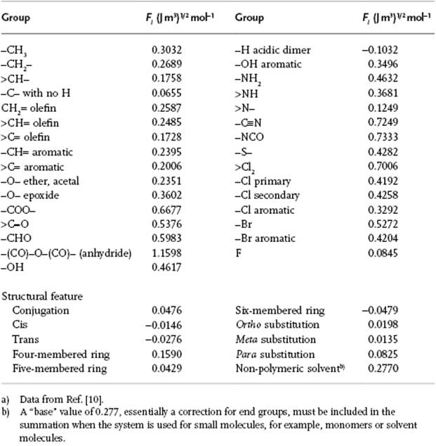
where ρ is the (mass) density of the amorphous polymer and M0 the molar mass of the repeating unit. The contributions Fi are tabulated for various chemical groups in the repeating unit, and a selection is given in Table 13.3 using the parameterization of Hoy [9]. A similar approach is used for random copolymers. One then takes δc = Σiδiwi, where δi and wi represent the delta and weight fraction of the repeating unit i in the copolymer. For alternating copolymers one takes the copolymer repeating unit as the monomer, but for block copolymers and grafted copolymers no satisfactory methods are available. For solvents, the group contribution approach is also applicable, but a small correction for end effects is usually applied (Table 13.3).
Table 13.3 Group contribution for the calculation of the solubility parameter.a)
For mixtures, one usually uses the rule-of-mixtures given by
(13.71) ![]()
where ϕ1 (δ1) and ϕ2 (δ2) represent the volume fraction (solubility parameter) of components 1 and 2. Further, one usually assumes that the temperature dependence of δ can be neglected, with most tables providing data for δ at 25 °C.
If the difference in solubility parameters Δδ = |δ2 − δ1| between two components is sufficiently small, the components are soluble in each other; otherwise a two-phase system results. For “normal” systems – that is, for systems without hydrogen bonding – a value of about Δδ = 4 (J m3)1/2 is often used.
Example 13.1
Calculate the δ-value for polystyrene (PS), –(CH2–CHC6H5)n.
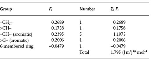
The density ρ = 1050 kg m−3 and M0 = 0.104 kg mol−1. Hence δ = ρΣiFi/M0 = 1050 × 1.795/0.104 = 18.1 MPa1/2. Testing whether PS dissolves in n-hexane, one needs ρ = 654 kg m−3 and M0 = 0.0861 kg mol−1, while ΣiFi = 1.957. Therefore δ = 14.7 MPa1/2. Hence, PS should dissolve in n-hexane, as in fact it does.
As might be expected, the above-described method – often denoted as the Hildebrand solubility parameter approach – is not suitable for use outside its original area, which is nonpolar, non-hydrogen-bonding solvents. Several attempts have been reported to extend and improve upon this scheme (see, e.g., van Krevelen [10]). One frequently used approach is that of Hansen [11]; whereas, in the original approach essentially only the dispersion forces were considered, Hansen divided the cohesive energy δ2 into three parts, namely
(13.72) ![]()
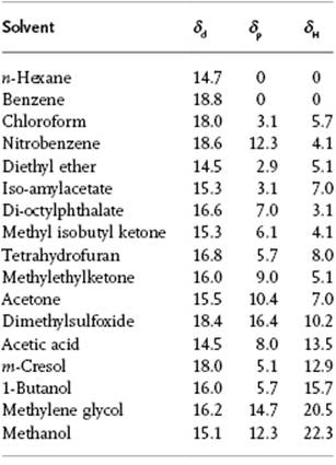
where the subscripts d, p, and H refer to the contributions due to dispersion forces, polar forces, and hydrogen bonding, respectively. From the experimental solubility data for many solvents, the parameters δd, δp and δH are determined using a least-squares approach. Data for a number of solvents are given in Table 13.4.
Table 13.4 The δ-parameters for several solvents in (MPa)1/2.
Using the values so obtained, one can again estimate whether two solvents are miscible, this being the case if the resulting value for δ2 − δ1 is sufficiently small. One can also “compose” in this way a solvent mixture with desired properties. For polymers, there is an extra parameter R0 that describes the radius of the “solubility sphere” in 2δd-δp-δH space. Hence, if ![]() , component 1 is a solvent for component 2 (the polymer), whereas when
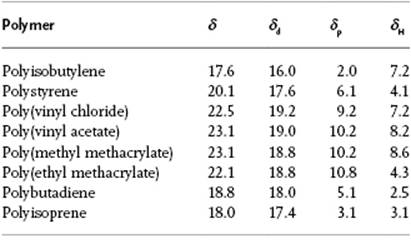
, component 1 is a solvent for component 2 (the polymer), whereas when ![]() , component 1 is a non-solvent for the polymer. The factor of 2 in front of the dispersion term has been the subject of debate. Whilst there is some theoretical basis [11, 12] for this factor, it was mainly introduced to match the experimental data. However, there are clearly systems [13] where the regions of solubility are far more eccentric than predicted by the standard Hansen theory. Values of δd, δp and δH for a number of polymers are reported in Table 13.5.
, component 1 is a non-solvent for the polymer. The factor of 2 in front of the dispersion term has been the subject of debate. Whilst there is some theoretical basis [11, 12] for this factor, it was mainly introduced to match the experimental data. However, there are clearly systems [13] where the regions of solubility are far more eccentric than predicted by the standard Hansen theory. Values of δd, δp and δH for a number of polymers are reported in Table 13.5.
Table 13.5 The δ-parameters for several polymers in (MPa)1/2 [10].
Although the Hildebrand parameter for non-polar solvents is usually close to the Hansen value, the latter has a wider applicability area. A typical example is provided by the fact that two solvents, butanol and nitroethane, which have the same Hildebrand parameter, are each incapable of dissolving typical epoxy polymers. Yet, a 50 : 50 mix is a good solvent for epoxy polymers. This can be easily explained by the fact that the Hansen parameters for this mix are close to the Hansen parameter of epoxy polymers.
The need to use a “matching factor” for the dispersion component clearly shows the semi-empirical nature of the whole scheme, in which many approximations are made. Yet, in spite of this, the approach is – practically speaking – rather useful, and estimates of the χ parameters often are reasonably accurate.
Problem 13.8
Verify the dimension of the molar attraction constant F in Table 13.3.
Problem 13.9
Calculate the solubility parameter of toluene from its vaporization enthalpy ΔvapH. To estimate ΔvapH, use the empirical rule that relates ΔvapH of a liquid to its boiling temperature Tn according to ![]() . For toluene: M = 92, ρ = 867 kg m−3, Tn = 383.7 K at 1 atm.
. For toluene: M = 92, ρ = 867 kg m−3, Tn = 383.7 K at 1 atm.
Problem 13.10
Calculate the solubility parameter δ of toluene from the group molar attraction constants Fi.
Problem 13.11
Calculate the composition by volume of a blend of n-hexane, t-butanol and dioctyl phthalate (use indices 1, 2, and 3 for these liquids for convenience) that would have the same solvent properties as tetrahydrofuran (use Table 13.4 and match δp and δH values). Use an equation analogous to Eq. (12.22) to assess the d, p, and H parts of the solubility parameter for solvent mixtures.