Liquid-State Physical Chemistry: Fundamentals, Modeling, and Applications (2013)

13.3. The Flory–Huggins Model

Let us now turn to the thermodynamics of polymer solutions. In 1941, Flory [3] and Huggins [4] published their (in the meantime) classic papers on the solutions of polymers. The principle of dealing with the problem remains the same as for molecular solutions: calculate the entropy of mixing Δ_mixS, the enthalpy of mixing Δ_mixH, and from these two quantities the Gibbs energy of mixing Δ_mixG. If Δ_mixG < 0, the polymer is soluble in the solvent. In this section we deal with this approach, using again the lattice model with coordination number z and having n sites, based on the original discussion of Flory [5] and the more recent version provided by Gedde [6]. As usual, we refer to component 1 as the solvent, and component 2 as the polymer.

13.3.1 The Entropy

The basis of the thermodynamic estimates for polymeric solutions is similar to that of molecular solutions (Figure 13.6). For molecular solutions, we have seen that the entropy of mixing was given by (see Section 11.4)

(13.36)

where, as before, n_i and x_i represent the number of moles and the mole fraction of component i, respectively, while R represents the gas constant. This expression can also be written (because it is assumed that for the molar volumes we have ) as:

(13.37)

where ϕ_i represents the volume fraction of component i. In Chapter 11, arguments were advanced to show that the proper expression is indeed in volume fractions.

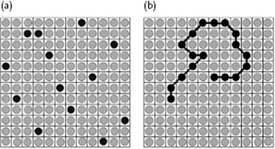
Figure 13.6 Lattice models for (a) molecular and (b) polymeric solutions.

Here, we derive the entropy expression for a polymer solution. In fact, in one set of considerations we can derive the relevant expressions not only for solutions but also for polymer blends and molecular solutions. To that purpose, we deal with solvent and solute on a symmetrical basis. We introduce first a reference volume V₀ that represents the molar volume of a lattice site which can be chosen arbitrarily, for example, V₀ = V₁, V₂ or (V₁V₂)^1/2. Often, one takes for V₀ the molar volume of the pure solvent . In the sequel we will also use the molecular reference volume v₀ = V₀/N_A where, as usual, N_A represents Avogadro's constant. Assuming no volume change, for a volume V_j of component j, the total volume of the solution is V = V₁ + V₂, and the number of sites⁵⁾ is n = V/v₀. Of these sites a volume fraction ϕ_j = V_j/V is occupied by component j, and therefore V_j/v_ref = nϕ_j.

Now, consider a molecule which in terms of the equivalent chain consists of r segments. If the molecular volume v_j of component j is given by v_j = V_j/N_A, the degree of polymerization is defined by r_j = v_j/v₀ = V_j/V₀ = M_j/ρ_jV₀, where M_j is the molar mass of the molecule that has density ρ_j (volume V_j) in the amorphous state at the solution temperature. Because v_j = r_jv, the number of molecules n_j of component j is n_j = V_j/v_j = V_j/r_jv₀ = nϕ_j/r_jv₀. Hence, on the lattice r₁n₁ sites are occupied by solvent molecules and r₂n₂ sites by polymer molecules, and the total number of lattice sites is n = r₁n₁ + r₂n₂.

We now turn again to solutions and use r₁ = 1 and r₂ = r. The analysis starts with having already i polymer molecules on the lattice, so that the number of vacant sites is then n − ir. This number equals the number of different ways of placing the (i + 1)th molecule on the lattice, which equals the product of the coordination number z and the fraction of remaining vacancies (1 − f_i), that is, z(1 − f_i). The next segment can only occupy (z − 1) (1 − f_i) positions. The number of different ways of arranging the (i + 1)th molecule is then

(13.38)

The number of ways to arrange all polymer molecules is accordingly

(13.39)

where the denominator n₂! takes into account that the solute molecules are indistinguishable. The fraction vacant sites is (1 − f_i) = (n − ir)/n which, upon substitution in Eq. (13.38), meanwhile replacing once z by z − 1, results in

(13.40)

Since we consider only diluted solutions, we have n >> r and therefore we can approximate Eq. (13.40) by

(13.41)

Substitution of Eq. (13.41) in Eq. (13.39) results in

(13.42)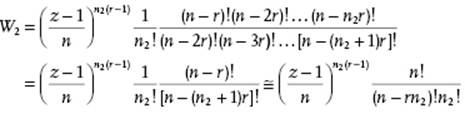

where the last step can be made only for dilute solutions with n >> r.

The entropy becomes S = klnW₂ which, upon some straightforward evaluation, using Stirling's approximation (lnx! = xlnx − x) and the fact that n = n₁ + n₂r, becomes

(13.43)

The entropy difference upon dissolution is calculated as ΔS = S(n₁,n₂) − S(0,n₂) because S(0,n₂) = kn₂lnr + kn₂(z − 1)ln[(z − 1)/e] represents the entropy of the amorphous polymer. Considering that the volume fractions of the solvent and solute are ϕ₁ = n₁/(n₁ + rn₂) and ϕ₁ = rn₂/(n₁ + rn₂), respectively, the result is (after some algebra)

(13.44)

Using n = n₁ + rn₂, the entropy change per site becomes Δ_mixS/n (note that Δ_mixS/n is an intensive quantity), so that Δ_mixS/nv₀ represents the entropy change per unit volume

(13.45)

The entropy expression also applies if both components are polymers, that is, for a blend. In this case we use again r_j = M_j/ρ_jV₀ leading to volume fractions given by

(13.46)

The entropy change per unit volume then becomes

(13.47)

and this quantity, since ϕ ≤ 1, is always positive. From these equations we conclude that, in the case of a polymer blend, the entropy gain per unit volume is relatively small as compared to that of the polymer solution because, in the former case n₁ = (ϕ₁Σ_jn_jr_j/r₁) is much smaller. Note that, if r₁ = r₂ = 1, we regain the ideal solution entropy. We included here only the mixing entropy, due to the translational degrees of freedom, and assumed that the configurational contribution would remain the same as for the pure polymer. Although this assumption is appropriate for blends, we discussed that excluded volume interactions for solutions have a significant influence. Moreover, we neglected volume changes which, although small, are actually present.

Problem 13.3

Estimate for which size ratio the volume fraction expression for the entropy deviates by more than 5% from the mole fraction expression.

13.3.2 The Energy

For the energy we must calculate the interaction between the solvent and solute segments, and we do this in a rather similar fashion to that used for molecular solutions. In particular, we neglect (again) volume changes and assume that the segments are placed at random over the lattice, thereby neglecting all correlation between segments. We again use a lattice of n sites with coordination number z and n₁ solvent molecules and n₂ polymer molecules, so that n = n₁ + rn₂. Each solute segment is surrounded by zϕ₁ solvent molecules and zϕ₂ solute segments, and therefore the interaction energy for that segment reads zϕ₁w₁₂ + zϕ₂w₂₂. Because the lattice contains nϕ₂ segments, each interacting in this way, the energy U₂ for the solute becomes

(13.48)

where the factor ½ is introduced to avoid counting interactions twice. Similarly, for the solvent molecules we obtain the energy

(13.49)

The energy for the pure solvent and solute are U₀₁ = ½nϕ₁zw₁₁ and U₀₂ = ½nϕ₂zw_22, respectively, so that the energy difference upon dissolution is calculated as

(13.50)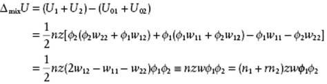

where w ≡ w₁₂ − ½(w₁₁ + w₂₂) is the interchange energy, the increase in energy when a solvent–polymer contact is formed from molecules that were originally contacting molecules of the same type.

In Flory–Huggins theory it is conventional to render the interaction parameter w dimensionless according to χ = zw/kT, where χ (chi) is the dimensionless interaction parameter. Values for many polymers are listed in handbooks [7]. Since ϕ₁ = n₁/(n₁ + n₂r₂), we can also write

(13.51)

The total volume of the solution is V = nv₀ = (n₁ + n₂r)v₀, where v₀ is the reference volume. The energy of mixing per unit volume then becomes

(13.52)

13.3.3 The Helmholtz Energy

From the entropy and energy, we obtain the Helmholtz energy

(13.53)

For the case of mixture of two polymers we obtain the result

(13.54)

with, as before, the DP r_j = M_j/ρ_jV₀. Note that the value of χ depends on the choice of V₀. Remembering that χ contributes to the Helmholtz energy, one should not be surprised that χ is temperature-dependent. Often, one writes

(13.55)

using the “entropic” and “enthalpic” parameters A and B, respectively, comparable to zw = a + bT, Eq. (11.75), for regular solutions. A typical example is the system polystyrene (PS)/polymethyl methacrylate (PMMA) with A = 0.0129 and B = 1.96 K using v₀ = 100 ų, resulting in χ ≅ 0.01, so that only low-molar mass components form a miscible blend. Empirically, this relationship is not generally observed, that is, the graph of χ versus 1/T may show curvature, local minima or even change sign, and is somewhat dependent on composition and chain length. Finally, we note that, as expected, for r₁ = r₂ = 1, we regain the regular solution description.

13.3.4 Phase Behavior

From the Helmholtz energy expression one can calculate the stability of the polymer solution via the conventional route, as used before for molecular (regular) solutions (see Eqs 11.67 to 11.70) which led in that case to kT_cri = ½zw. Here, the main result for a binary polymer mixture with ϕ₁ = ϕ and ϕ₂ = 1 − ϕ, is

(13.56)

Equating this result to zero, one obtains the expression for the inflection points of the Helmholtz curve, dependent on composition and separating unstable and metastable regions. It is conventionally labeled as the spinodal (line) (see Sections 16.1 and 16.2), and reads for this case

(13.57)

Using χ = A + B/T one obtains

(13.58)

The critical point corresponds to the minimum in this curve and is obtained from

(13.59)

which corresponds to the critical composition

(13.60)

and upon substitution this result in the spinodal to

(13.61)

Since n₂ is usually large this implies for solutions (n₁ = 1) that, in the limit of infinite molar mass, χ_cri = ½ or kT_cri = 2zw, in contrast to the result for regular solutions kT_cri = ½zw. For the most common case where B > 0, χdecreases with increasing T and the solubility increases. The highest temperature for a two-phase system to exist is the upper critical solution temperature (UCST) and for T > T_cri the homogeneous solution is stable. However, B < 0 also occurs and χ increases with increasing T so that the solubility decreases. The lowest temperature for a homogeneous solution to exist is the lower critical solution temperature (LCST). If B changes sign as a function of T, the system will show both an UCST and a LCST.

In order to be able to describe the UCST, both the “entropic” part A and “enthalpic” part B can be considered to be temperature-independent. From Problem 13.5 we have

(13.62)

so that for the DP r₂ ≡ r → ∞, χ_cri = ½. Combining with χ = A + B/T and solving for T_cri(r = ∞) ≡ θ, we obtain ½ = A + B/θ and therefore

(13.63)

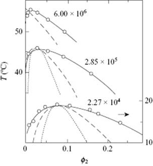
describing 1/T_cri as a function of θ and r. Hence, given a set of experimental values of T_cri as a function of r, the slope of Eq. (13.63) determines B and the intercept determines θ, and therefore A. An example is shown in Figure 13.7.

Figure 13.7 Experimental and calculated phase diagrams for three polyisobutylene fractions in diisobutyl ketone of the molecular weights indicated. The dashed curves are the calculated Flory–Huggins binodals, while the dotted curves are the spinodals. The model description is due to Casassa [37], using the data of Schultz and Flory [38].

The temperature θ can be shown to be indeed the theta temperature. From Problem 13.6 we have, remembering that a₁ = γ₁x₁ and that ϕ₁ = 1 − ϕ₂,

(13.64)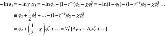

where in the third line r → ∞ is used. In the last step we apply an expansion similar to that used for the osmotic pressure (see Section 13.2), but now for lna₁ instead of the osmotic factor g. The concentration of the polymer is given by c₂ = n₂M₂/V, where n₂ is the number of moles of polymer of molecular mass M₂ in a volume V. If we assume that we have no volume change upon mixing, the volume of the polymer V₂ is given by , with the specific volume of the pure polymer as defined by , so that . The Flory–Huggins first and second osmotic virial coefficients A₁ and A₂ become, respectively,

(13.65)

Similarly to what is discussed in Section 11.3, the first osmotic virial coefficient A₁ is determined entirely by the molecular mass M₂. From Eq. (13.65) we see further that A₂ vanishes if χ = ½ and the solution behaves to third order as an ideal solution, that is, the chains are “unperturbed.” This behavior is comparable to the pseudo-ideal pressure behavior of gases at the Boyle temperature, where the second virial coefficient vanishes. We have already indicated that for r → ∞, χ_cri = ½, and therefore it is appropriate to consider θ as the theta temperature.

In the spirit of the osmotic expansion, we expect that the second osmotic virial coefficient A₂ characterizes the onset of intermolecular interactions between the polymer solute molecules, and therefore depends on M₂. However, we predict that A₂ is independent of M₂, which experimentally is not the case. This shows one of the deficiencies of the Flory–Huggins model, namely that it is not valid for very dilute systems because the assumption that a segment experiences the interaction for a random distribution of segments and solvent molecules cannot be true for such a solution.

Let us now consider the LCST. Whereas, for the UCST the parameters A and B could be considered as temperature-independent, when describing the LCST they should be considered as temperature-dependent. This can be done, for example, by writing

(13.66)

with ΔC_P the exchange heat capacity. Using the Gibbs–Helmholtz equation, we obtain

(13.67)

If ΔC_P is considered as constant, we easily evaluate this expression to

(13.68)

If we accept that it is possible that ΔC_P < 0, χ as a function of T shows a minimum and two critical temperatures exist: T = θ, representing the UCST, and another temperature representing the LCST. Typical values of ΔC_P required are ΔC_P ≅ −k to −2k. One interpretation for ΔC_P < 0 is that the interchange energy between solute segments and solvent molecules becomes lower as the system expands with increasing temperature.

Some further aspects of the FH theory are discussed by Boyd and Phillips [1].

Problem 13.4: Asymmetry

Plot Δ_mixF as resulting from the Flory–Huggins theory with χ = 1, 2, and 3 for:

a) r₁ = 1 and r₂ = 1, 10, 10², and 10⁴.

b) r₁ = 10² and r₂ = 10² and 10⁴.

c) r₁ = 10⁴ and r₂ = 10⁴.

Problem 13.5: Phase separation

Using the Flory–Huggins expression Eq. (13.54) as well as r₁ = 1 and r₂ = r:

a) Show that the critical values of ϕ₂ and χ for phase separation to occur in polymer solutions are given by, respectively,

Check that χ_cri = ½ for infinite molecular mass of the polymer.

b) Show that the critical temperature T_cri can be described by

Problem 13.6: Activity coefficient

Show by using Eq. (11.9) that the activity coefficients of the solvent (1) and the polymer (2) containing r monomers per polymer in the Flory–Huggins model are given by, respectively,

Problem 13.7: LCST

Derive Eq. (13.68).