Physical Chemistry Essentials - Hofmann A. 2018

Solutions of Electrolytes
4.1 Fundamental Concepts

4.1.1 Ions in Solution

In the previous sections, we have mostly assumed that the systems under study consisted of non-dissociating solutes, i.e. non-electrolytes. We now want to expand considerations to substances that dissociate in solution. Such substances are called electrolytes and form ions when being dissolved in solvents. Electrolytes can be classified into strong and weak electrolytes.

Strong electrolytes completely dissociate in solution:

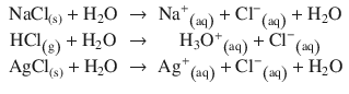
In contrast, weak electrolytes do not fully dissociate in solution, due to inter-ionic interactions:

The occurrence of ions in solutions of electrolytes is not dependent on the flow of current; electrolytes dissociate readily upon dilution in solvent. The degree of dissociation α (see Sect. 4.3.3) describes the fraction of solute present as ions.

In aqueous solution, ions have water molecules associated with them; this is called the hydration shell. Ions change the structure of the water hydrogen bond network. In the presence of an ion, a water molecule reorients such that its polarised charge faces the opposite charge of the ion. During this reorientation process, the hydrogen bonds of the water molecule to its nearest neighbours is broken. The orientation of the water molecules that form the hydration shell directly around the ion is called the inner solvation shell (see Fig. 4.1, orange molecules) and results in a net charge on the outside of this shell. This charge is of the same sign as that of the ion in the centre. The charge on the outside of this inner hydration shell causes further water molecules in the vicinity to reorient, leading to a second solvation shell (see Fig. 4.1, red molecules).

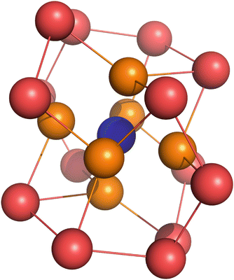
Fig. 4.1

Quantum-chemical calculations with the semi-empirical AM1 method show that mono-atomic ions (such as e.g. Na⁺, blue) exist in a hydration shell resulting in the complex [Na(OH₂)₂₀]⁺ (Peslherbe et al. 2000). The shell consists of an inner solvation shell where six water molecules take the vertex positions of an octahedron (orange). The remaining 14 water molecules (red) form the second solvation shell. The water structure around the cation takes the form of a puckered dodecahedron. The formation of this structure can be thought of as a ’pulling in’ of the inner solvation shell molecules from their initial positions on the vertices of a regular dodecahedron

The occurrence of such hydration shells explains the freezing point depression of solutions. The hydration shells of dissolved ions disrupt the hydrogen bonding network of water that would otherwise form the hexagonal structure of ice.

4.1.2 Charge and Electroneutrality

The charge Q describes the quantity of electricity; it can be positive (cations, protons) or negative (anions, electrons). The charge is measured in units of Coulomb: [Q] = 1 C.

The elementary charge is the charge of the electron: |Q(e⁻)| = e = 1.602 · 10⁻¹⁹ C.

If matter possesses only fixed charges, then it is called an insulator. In contrast, the existence of mobile charges makes matter a conductor. In case of an electronic conductor, the mobile charges are electrons, in ionic conductors, the mobile charges are ions. Some examples are given in Table 4.1. In solutions, ions represent the moving charges and are thus responsible for conducting electricity.

Table 4.1

Examples of different types of conductors

The principle of electroneutrality states that there can be no significant net charge in any macroscopic volume within a conductor. This is a consequence of the work required to separate opposite charges, or to bring like charges into close contact. This work raises the free energy change of the underlying process that may lead to unbalanced charges, thus making it less spontaneous. The amount of unbalanced charges that is allowed is due to different concentrations of oppositely charged species that are not chemically significant (and thus results in differences in the electric potential of no more than a few volts; see Sects. 4.1.4 and 4.2.3).

4.1.3 Electric Current

Current (I) is the flow of charge dQ in a particular time interval dt through a defined volume:

(4.1)

If we consider charges moving through a cylindrical wire (Fig. 4.2), we can calculate the amount of charge dQ passing through a cylindrical volume element during the time interval dt by counting the number of passing charges (N _passing) and multiply with the unit charge e as well as the charge state z:

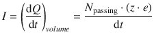
(4.2)

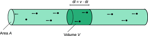
Fig. 4.2

Mobile charges passing through a cylindrical volume element V. The cylinder has a cross-section area A. The length dl of the volume element is given by the speed v of the charges multiplied with the time interval dt

By multiplying and diving with the volume V of the volume element and substituting

we obtain:

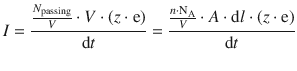
We can further substitute

which yields

This simplifies to:

(4.3)

F is the Faraday constant and has the value of:

Equation 4.3 provides a relation between the current and the molar concentration c of charged particles with the charge state z that move with the speed v.

4.1.4 Electric Potential

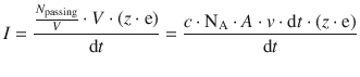
Figure 4.3 shows the scheme of a simple electric circuit where a direct current power supply gives rise to electrons moving from the cathode (excess of electrons) to the anode (shortage of electrons) through a cylindrical wire. The fact that electrons move from the cathode to the anode can be conceptualised by the existence of a potential difference ΔE between the cathode and the anode. The potential difference ΔE is measured in units of volts:

Fig. 4.3

Illustration to derive the relationship between the potential difference ΔE, current I and the travelling parameters (length, cross-sectional area) of the moving charges

Whereas the physical movement of electrons has the direction cathode → anode, the current I is defined to flow in the opposite direction.

As in the previous section, we consider a volume element V in the cylindrical wire of Fig. 4.3; the volume of this element can be calculated from the cross-sectional area A and the length l, as per V = A·l.

It is obvious that there will be more current flowing, if the potential difference of the power supply is higher; I and ΔE will thus be proportional to each other. Because the potential difference between the anode and the cathode is taken as positive, and the current flows from the anode to the cathode, the directions of the two phenomena are opposite, hence:

(4.4)

If we increase the length l of the volume element, we will need to increase the potential difference ΔE to have the same amount of charges (i.e. the same current) flowing through that volume element. Therefore:

(4.5)

The opposite is true for the cross-sectional area A. If we widen the area A, but require the same amount of charges to flow through, the potential difference ΔE needs to be decreased. It thus appears that

(4.6)

It follows from Eqs. 4.4—4.6:

(4.7)

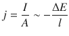
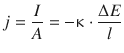
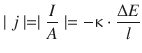
If we define a new quantity j called the current density as

(4.8)

then we obtain from Eq. 4.7:

(4.9)

As proportionality factor we introduce κ as the electric conductivity:

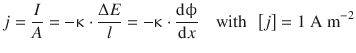
(4.10)

The potential difference ΔE over a distance l is called the electric field. The electric field is the gradient of the electric potential ϕ over a distance:

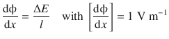
(4.11)

It follows that the conductivity κ is measured in units of siemens per metre:

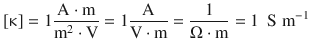
(4.12)

Since conductivity is a specific property of a substance, it lends itself as a quantity to distinguish conducting from insulating matter (see Table 4.2).

Table 4.2

Conductivity of different substances

4.1.5 Resistance

An important relationship for electric circuits (see Fig. 4.3) is that between the electric potential and the current flowing through the circuit. From Eq. 4.10 we can resolve an expression for the potential ΔE:

(4.10)

(4.13)

The quotient with the length l, the area A and the conductivity κ describes constants of a particular electric circuit and as such represents a material constant for the given system. This quotient is thus defined as the electric resistance R:

(4.14)

and Eq. 4.13 yields:

(4.15)

which constitutes Ohm’s law. The resistance is measured in units of ohm: [R] = 1 Ω.

The electric resistance of a conductor represents the opposition to the passage of charges through that conductor. Intuitively, the willingness of a conductor to let charges pass through will be a quantity that is inversely related to the resistance. The quantity describing the ease with which charges can pass through is called the conductance G:

(4.16)

The conductance is measured in units of siemens: [G] = 1 Ω⁻¹ = 1 S. Like the resistance, the conductance is a property of the conductor used in the electric circuit.

4.1.6 Conductivity and Conductance

The electric conductivity κ is the ratio between the current density and the electric field (Eq. 4.10). As such, it is a property of the conducting material. In contrast, the conductance G describes the current-carrying capacity of the electrolytic substance; in solutions of electrolytes, the conductance is thus a property of the dissolved ions. The conductance of electrolytic solutions increases with dilution for both strong and weak electrolytes, because at low concentration there is less hindrance for the migrating ions from neighbours.

The specific conductance g measures the current-carrying capacity of all ions in a specific volume:

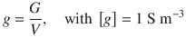
(4.17)

For strong electrolytes, the specific conductance decreases with dilution.

Whereas the conductance G depends on the physical size of the conductor, the conductivity κ is independent of the conductor size. Conductivity and conductance are related as per:

(4.10)

With it follows:

(4.18)

The conductance of a system is therefore equal to the conductivity of this system, multiplied by the area through which the migrating charges pass, and divided by the distance travelled.