Physical Chemistry Essentials - Hofmann A. 2018

Intermolecular Interactions
12.1 Interactions of Permanent Dipoles

In the preceding chapter, we discussed the various types of chemical bonds that are holding individual atoms together such as to build up new entities—molecules (or metals). These new entities possess different characteristics and functions than the individual atoms they comprise of. Molecules can engage in further interactions, which is the subject of this chapter.

The strength of interaction decreases in the following three phenomena in the order of their discussion: the interactions of permanent dipoles is stronger than interactions involving induced dipoles. The weakest interaction thus arises from interactions exclusively between induced dipoles, the so-called London dispersion force. The combined interactions involving dipoles constitute the van der Waals interactions (or van der Waals bond) which has been discussed in Sect. 11.5. For consistency, we continue to denote the potential energy as V in the following sections in order to avoid confusion with the electric field E. The dipole moment has been introduced in Sect. 11.3.5.

The hydrogen bond gives rise to a much stronger, but still non-covalent, interaction between two molecules. This type of interaction occurs when a hydrogen atom is bound to a highly electronegative (see Sect. 11.2) atom such as nitrogen, oxygen or fluorine. Coulomb interactions are electrostatic interactions and have been discussed when introducing the ionic bond (Sect. 11.1).

12.1 Interactions of Permanent Dipoles

12.1.1 Dipole—Dipole Interactions

Polar molecules are characterised by a localisation of charges in different parts of the molecule. Frequently, the value of charges separated is smaller than the fundamental charge e, i.e. the localised charges are partial charges (denoted by δ+ and δ−). This charge separation constitutes a permanent dipole and such molecules may interact with each either through attractive electrostatic interactions.

For two molecules with dipole moments μ_A and μ_B, respectively, many different relative orientations (with attractive as well as repulsive interactions) of the two dipoles are possible. Four extreme cases of orientations with attractive/repulsive interactions are shown in Fig. 12.1.

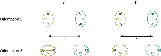
Fig. 12.1

Extreme orientations of two permanent dipoles for attractive (a) and repulsive (b) interactions

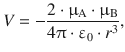
In orientation 1A, the interaction energy (potential energy) is

(12.1)

and in orientation 2A, the energy is:

(12.2)

whereby ε₀ is the permittivity in vacuo and r the distance between the two dipoles. Note that the negative sign in Eqs. 12.1 and 12.2 relates to the directions of the dipole moments as shown in Fig. 12.1. The interaction energy assumes negative values and hence describes an attraction. If the direction of one of the dipole moments is reversed (orientations 1B and 2B in Fig. 12.1), the negative sign in above equations needs to be reversed to, which makes the interaction energy positive and thus describes a repulsion.

If we consider a bulk system of above molecules, it would appear at a first glance that all possible orientations are populated and the mean interaction energy was zero, since the attractive and repulsive interactions cancel each other in the sum. However, due to the Maxwell—Boltzmann statistics (see Sect. 5.1.2), orientations with favourable interactions outweigh those with unfavourable interactions with a factor that is proportional to

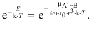
Averaged over all rotational orientations of the two dipole moments μ_A and μ_B, the interaction energy of two permanent dipoles, the interaction energy between the two dipoles has been derived by Willem Hendrik Keesom (1915). The interactions between two permanent dipoles are thus also known as Keesom interactions and their interaction (potential) energy is inversely proportional to the sixth power of r, i.e. it falls of rapidly with increasing distance:

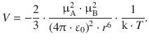
(12.3)

The above relationship also shows that the interaction energy decreases with increasing temperature. This is to be expected, since the molecules (=permanent dipoles) possess higher kinetic energy at higher temperatures which prevents the spatial alignment of dipole moments required for favourable interactions.

12.1.2 Ion—Dipole Interactions

The interactions between ions and permanent dipoles are an important characteristic of aqueous solutions. Water is a highly polar molecule with a dipole moment of 1.8 D. In the presence of cations (e.g. Na⁺), the water dipoles are arranged around the cations such that their negative (oxygen) ends point towards the cation. Similarly, around an anion (e.g. Cl⁻), the dipoles are oriented with their positive (hydrogen) ends pointing towards the anion. Due to these attractive interactions, ions in aqueous solutions are always hydrated.

12.2 Interactions of Temporary Dipoles

Neutral, non-polar atoms or molecules possess no localised electrical charge or permanent dipole moment (i.e. no separated partial charges). However, the approach of an ion or a dipole induces a temporary dipole in the non-polar species. The interaction between the ion or dipole with the induced dipole results in an attractive interaction.

12.2.1 Ion—Induced Dipole Interactions

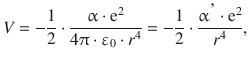
In Fig. 12.2, we consider an atom that possesses an electron density of spherical symmetry around the nucleus. The approach of a charged particle (e.g. a cation) distorts the electron density of the atom and induces a dipole. The magnitude of the induced dipole moment μ_ind depends on the properties of the atom (or chemical moiety) as well as the electric field elicited by the approaching charged particle. The ease with which an outside electric field can distort the electron density of the neutral species is called polarisability α. The interaction energy of ion—induced dipole interactions is then given by:

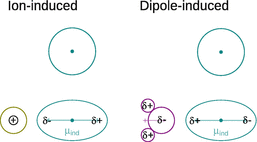
Fig. 12.2

Attractive interactions of ion-induced and dipole-induced temporary dipoles in a neutral atom. The dot indicates the position of the nucleus

(12.4)

where ε₀ is the vacuum permittivity and r the distance between the charged ion and the neutral species. We recall that the polarisability is the factor of proportionality between the field strength E and the induced dipole momentum μ_ind (see Sect. 11.5):

(11.18)

Often, the polarisability is expressed as a related quantity that is more suitable to the context in which it is determined. Frequently, it is the polarisability volume α′ which is given by

(12.5)

and has the units of a volume. Some polarisability-related quantities for H₂O are summarised in Table 12.1.

Table 12.1

Polarisability and related quantities for H₂O

In larger molecules, polarisability is typically assessed for individual groups, such as bonds or chemical functionalities. In general, larger groups with diffuse electron densities possess a higher polarisability than smaller groups with strongly located electrons. Highly polarisable groups therefore include

✵ anions,

✵ groups with π electron systems (e.g. phenyl group, nucleic acids, etc.),

✵ unsaturated bonds (e.g. C=C, C=N, nitro groups).

Generally, the polarisability of atoms depends on two factors. First, the polarisability of atoms with a large number of electrons is higher than those of atoms with a smaller number of electrons (the nuclear charge has less control on charge distribution the more electrons there are). Second, the more distant electrons are from the atomic nucleus, the less their localisation can be controlled by the nuclear charge; therefore, the polarisability increases the more distant electrons are located from the nucleus. The combination of both factors results in the observation that heavier atoms possess a higher polarisability, since heavier atoms possess more electrons and occupy more distant orbitals.

In molecules with an extended shape (this excludes tetrahedral, octahedral and icosahedral molecules), the orientation with respect to an electric field can also affect the polarisability. Higher polarisability in such molecules (e.g. 2,4-hexadiene) is achieved when the electric field is applied parallel rather than perpendicular to the molecule.

12.2.2 Dipole—Induced Dipole Interactions

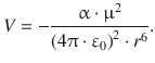
A permanent dipole can also distort the electron distribution of a neutral atom or non-polar molecule, and thereby induce a temporary dipole. This leads to an attractive interaction as illustrated in Fig. 12.2 and the interaction energy as derived by Peter Debye:

(11.19)

In above equation, ε is again the dielectric constant of the medium, r the distance between the two dipoles, α the polarisability of the non-polar molecules and μ the dipole moment of the permanent dipole.

The interaction between permanent and induced dipoles is also known as the Debye force. Importantly, in contrast to the interactions of permanent dipoles (Keesom interactions), the interactions involving induced dipoles is not dependent on the temperature. Since the temporary dipoles can be induced instantaneously, the thermal motion of the molecules does not affect this interaction.