Advanced Calculus of Several Variables (1973)
Part II. Multivariable Differential Calculus
Chapter 2. DIRECTIONAL DERIVATIVES AND THE DIFFERENTIAL
We have seen that the definition of the derivative of a function of a single variable is motivated by the problem of defining tangent lines to curves. In a similar way the concept of differentiability for functions of several variables is motivated by the problem of defining tangent planes to surfaces.
It is customary to describe the graph in ![]() 3 of a function f :
3 of a function f : ![]() 2 →
2 → ![]() as a “surface” lying “over” the xy-plane
as a “surface” lying “over” the xy-plane ![]() 2. This graph may be regarded as the image of the mapping F :
2. This graph may be regarded as the image of the mapping F : ![]() 2 →
2 → ![]() 3 defined by F(x, y) = (x, y, f(x, y)). Generalizing this geometric interpretation, we will (at least in the case m > n) think of the image of a mapping F :
3 defined by F(x, y) = (x, y, f(x, y)). Generalizing this geometric interpretation, we will (at least in the case m > n) think of the image of a mapping F : ![]() n →
n → ![]() m as an n-dimensional surface in
m as an n-dimensional surface in ![]() m. So here we are using the word “surface” only in an intuitive way; we defer its precise definition to Section 5.
m. So here we are using the word “surface” only in an intuitive way; we defer its precise definition to Section 5.
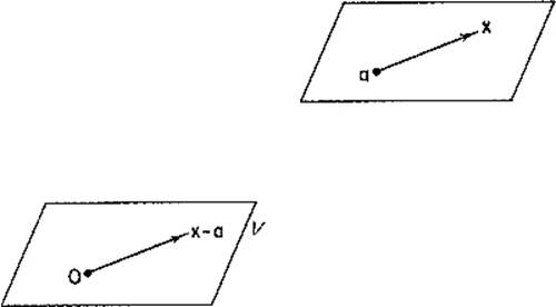
Figure 2.5
One would naturally expect an n-dimensional surface in ![]() m (m > n) to have at each point an n-dimensional tangent plane. By an n-dimensional plane in
m (m > n) to have at each point an n-dimensional tangent plane. By an n-dimensional plane in ![]() m will be meant a parallel translate of an n-dimensional subspace (through the origin) of
m will be meant a parallel translate of an n-dimensional subspace (through the origin) of ![]() m. If V is a subspace of
m. If V is a subspace of ![]() m, by the parallel translate of V through the point
m, by the parallel translate of V through the point ![]() (or the parallel translate of V to a) is meant the set of all points
(or the parallel translate of V to a) is meant the set of all points ![]() such that
such that ![]() (Fig. 2.5). If V is the solution set of the linear equation
(Fig. 2.5). If V is the solution set of the linear equation
![]()
where A is a matrix and x a column vector, then this parallel translate of V is the solution set of the equation
![]()
Given a mapping F : ![]() n →
n → ![]() m and a point
m and a point ![]() , let us try to define the plane (if any) in
, let us try to define the plane (if any) in ![]() m that is tangent to the image surface S of F at F(a). The basic idea is that this tangent plane should consist of all straight lines through F(a) which are tangent to curves in the surface S (see Fig. 2.6).
m that is tangent to the image surface S of F at F(a). The basic idea is that this tangent plane should consist of all straight lines through F(a) which are tangent to curves in the surface S (see Fig. 2.6).
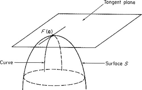
Figure 2.6
Given ![]() , we consider, as a fairly typical such curve, the image under F of the straight line in
, we consider, as a fairly typical such curve, the image under F of the straight line in ![]() n which passes through the point a and is parallel to the vector v. So we define γv :
n which passes through the point a and is parallel to the vector v. So we define γv : ![]() →
→ ![]() m by
m by
![]()
for each ![]() .
.
We then define the directional derivative with respect to v of F at a to be the velocity vector γv′(0), that is,
![]()
provided that the limit exists. The vector Dv F(a), translated to F(a), is then a tangent vector to S at F(a) (see Fig. 2.7).
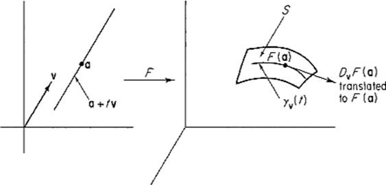
Figure 2.7
For an intuitive interpretation of the directional derivative, consider the following physical example. Suppose f(p) denotes the temperature at the point ![]() . If a particle travels along a straight line through p with constant velocity vector v, then Dvf(p) is the rate of change of temperature which the particle is experiencing as it passes through the point p (why?).
. If a particle travels along a straight line through p with constant velocity vector v, then Dvf(p) is the rate of change of temperature which the particle is experiencing as it passes through the point p (why?).
For another interpretation, consider the special case f : ![]() 2 →
2 → ![]() , and let
, and let ![]() be a unit vector. Then Dvf(p) is the slope at
be a unit vector. Then Dvf(p) is the slope at ![]() of the curve in which the surface z = f(x, y) intersects the vertical plane which contains the point
of the curve in which the surface z = f(x, y) intersects the vertical plane which contains the point ![]() and is parallel to the vector v (why?).
and is parallel to the vector v (why?).
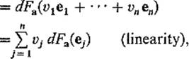
Of special interest are the directional derivatives of F with respect to the standard unit basis vectors e1, . . . , en. These are called the partial derivatives of F. The ith partial derivative of F at a, denoted by
![]()
is defined by
![]()
If a = (a1, . . . , an), we see that
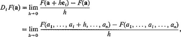
so DiF(a) is simply the result of differentiating F as a function of the single variable xi, holding the remaining variables fixed.
Example 1 If f(x, y) = xy, then D1 f(x, y) = y and D2 f(x, y) = x. If g(x, y) = ex sin y, then D1 g(x, y) = ex sin y and D2 g(x, y) = ex cos y.
To return to the matter of the tangent plane to S at F(a), note that
so Dv F(a) and Dw F(a) are collinear vectors in ![]() m if v and w are collinear in
m if v and w are collinear in ![]() n. Thus every straight line through the origin in Rn determines a straight line through the origin in
n. Thus every straight line through the origin in Rn determines a straight line through the origin in ![]() m. Obviously we would like the union
m. Obviously we would like the union
![]()
of all straight lines in ![]() m obtained in this manner, to be a subspace of Rm. If this were the case, then the parallel translate of
m obtained in this manner, to be a subspace of Rm. If this were the case, then the parallel translate of ![]() a to F(a) would be a likely candidate for the tangent plane to S at F(a).
a to F(a) would be a likely candidate for the tangent plane to S at F(a).
The set ![]() is simply the image of
is simply the image of ![]() n under the mapping L :
n under the mapping L : ![]() n →
n → ![]() m defined by
m defined by
![]()
for all ![]() . Since the image of a linear mapping is always a subspace, we can therefore ensure that
. Since the image of a linear mapping is always a subspace, we can therefore ensure that ![]() a is a subspace of
a is a subspace of ![]() m by requiring that L be a linear mapping.
m by requiring that L be a linear mapping.
We would also like our tangent plane to “closely fit” the surface S near F(a). This means that we want L(v) to be a good approximation to F(a + v) − F(a) when ![]() v
v![]() is small. But we have seen this sort of condition before, namely in Theorem 1.2. The necessary and sufficient condition for differentiability in the case n = 1 now becomes our definition for the general case.
is small. But we have seen this sort of condition before, namely in Theorem 1.2. The necessary and sufficient condition for differentiability in the case n = 1 now becomes our definition for the general case.
The mapping F, from an open subset D of ![]() n to
n to ![]() m, is differentiable at the point
m, is differentiable at the point ![]() if and only if there exists a linear mapping L :
if and only if there exists a linear mapping L : ![]() n →
n → ![]() m such that
m such that
![]()
The linear mapping L is then denoted by dFa, and is called the differential of F at a. Its matrix F′(a) is called the derivative of F at a. Thus F′(a) is the (unique) m × n matrix, provided by Theorem 4.1 of Chapter I, such that
![]()
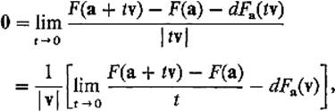
for all ![]() . In Theorem 2.4 below we shall prove that the differential of F at a is well defined by proving that
. In Theorem 2.4 below we shall prove that the differential of F at a is well defined by proving that
![]()
in terms of the partial derivatives of the coordinate functions F1, . . . , Fm of F. For then if L1 and L2 were two linear mappings both satisfying (4) above, then each would have the same matrix given by (6), so they would in fact be the same linear mapping.
To reiterate, the relationship between the differential dFa and the derivative F′(a) is the same as in Section 1—the differential dFa : ![]() n →
n → ![]() m is a linear mapping represented by the m × n matrix F′(a).
m is a linear mapping represented by the m × n matrix F′(a).
Note that, if we write ΔFa(h) = F(a + h) − F(a), then (4) takes the form
![]()
which says (just as in the case n = 1 of (Section 1) that the difference, between the actual change in the value of F from a to a + h and the approximate change dFa(h), goes to zero faster than h as h → 0. We indicate this by writing ΔFa(h) ≈ dFa(h), or F(a + h) ≈ F(a) + dFa(h). We will see presently that dFa(h) is quite easy to compute (if we know the partial derivatives of F at a), so this gives an approximation to the actual value F(a + h) if ![]() h
h![]() is small. However we will not be able to say how small
is small. However we will not be able to say how small ![]() h
h![]() need be, or to estimate the “error” ΔFa(h) − dFa(h) made in replacing the actual value F(a + h) by the approximation F(a) + dFa(h), until the multivariable Taylor's formula is available Section 7). The picture of the graph of F when n = 2 and m = 1 is instructive (Fig. 2.8).
need be, or to estimate the “error” ΔFa(h) − dFa(h) made in replacing the actual value F(a + h) by the approximation F(a) + dFa(h), until the multivariable Taylor's formula is available Section 7). The picture of the graph of F when n = 2 and m = 1 is instructive (Fig. 2.8).
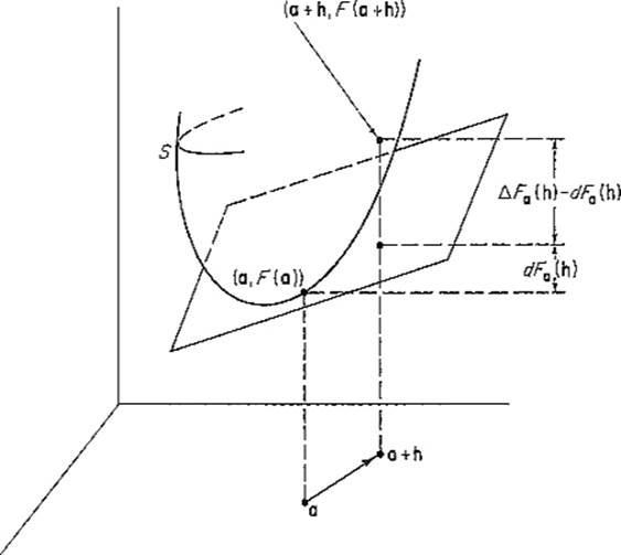
Figure 2.8
Example 2 If F : ![]() n →
n → ![]() m is constant, that is, there exists
m is constant, that is, there exists ![]() such that F(x) = b for all
such that F(x) = b for all ![]() , then F is differentiable everywhere, with dFa = 0 (so the derivative of a constant is zero as expected), because
, then F is differentiable everywhere, with dFa = 0 (so the derivative of a constant is zero as expected), because
![]()
Example 3 If F : ![]() n →
n → ![]() m is linear, then F is differentiable everywhere, and
m is linear, then F is differentiable everywhere, and
![]()
In short, a linear mapping is its own differential, because
![]()
by linearity of F.
For instance, if s : ![]() 2 →
2 → ![]() is defined by s(x, y) = x + y, then dsa = s for all
is defined by s(x, y) = x + y, then dsa = s for all ![]()
The following theorem relates the differential to the directional derivatives which motivated its definition.
Theorem 2.1 If F : ![]() n →
n → ![]() m is differentiable at a, then the directional derivative Dv F(a) exists for all
m is differentiable at a, then the directional derivative Dv F(a) exists for all ![]() , and
, and
![]()
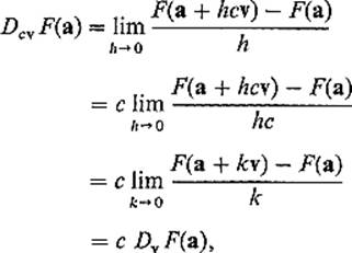
PROOF We substitute h = tv into (4) and let t → 0. Then
so it is clear that
![]()
exists and equals dFa(v).
![]()
However the converse of Theorem 2.1 is false. That is, a function may possess directional derivatives in all directions, yet still fail to be differentiable.
Example 4 Let f : ![]() 2 →
2 → ![]() be defined by
be defined by
![]()
unless x = y = 0, and f(0, 0) = 0. In Exercise 7.4 of Chapter 1 it was shown that f is not continuous at (0, 0). By Exercise 2.1 below it follows that f is not differentiable at (0, 0). However, if v = (a, b) with b ≠ 0, then
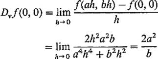
exists, while clearly Dvf(0, 0) = 0 if b = 0. Other examples of nondifferentiable functions that nevertheless possess directional derivatives are given in Exercises 2.3 and 2.4.
The next theorem proceeds a step further, expressing directional derivatives in terms of partial derivatives (which presumably are relatively easy to compute).
Theorem 2.2 If F : ![]() n →
n → ![]() m is differentiable at a, and v = (v1, . . . , vn), then
m is differentiable at a, and v = (v1, . . . , vn), then
![]()
PROOF
![]() (by Theorem 2.1)
(by Theorem 2.1)
so ![]() , applying Theorem 2.1 again.
, applying Theorem 2.1 again.
![]()
In the case m = 1 of a differentiable real-valued function f : ![]() n →
n → ![]() , the vector
, the vector
![]()
whose components are the partial derivatives of f, is called the gradient vector of f at a. In terms of ![]() f(a), Eq. (8) becomes
f(a), Eq. (8) becomes
![]()
which is a strikingly simple expression for the directional derivative in terms of partial derivatives.
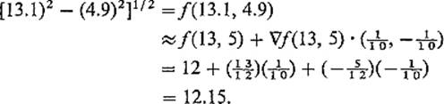
Example 5 We use Eq. (10) and the approximation Δfa(h) ≈ dfa(h) to estimate [(13.1)2 – (4.9)2]1/2. Let f(x, y) = (x2 − y2)1/2, a = (13, 5), ![]() . Then
. Then ![]() , so
, so
To investigate the significance of the gradient vector, let us consider a differentiable function f : ![]() n →
n → ![]() and a point
and a point ![]() , where
, where ![]() f(a) ≠ 0. Suppose that we want to determine the direction in which f increases most rapidly at a. By a “direction” here we mean a unit vector u. Let θu denote the angle between u and
f(a) ≠ 0. Suppose that we want to determine the direction in which f increases most rapidly at a. By a “direction” here we mean a unit vector u. Let θu denote the angle between u and ![]() f(a). Then (10) gives
f(a). Then (10) gives
![]()
But cos θu attains its maximum value of + 1 when θu = 0, that is, when u and ![]() f(a) are collinear and point in the same direction. We conclude that
f(a) are collinear and point in the same direction. We conclude that ![]()
![]() f(a)
f(a)![]() is the maximum value of Duf(a) for u a unit vector, and that this maximum value is attained with u =
is the maximum value of Duf(a) for u a unit vector, and that this maximum value is attained with u = ![]() f(a)/
f(a)/![]()
![]() f(a)
f(a)![]() .
.
For example, suppose that f(a) denotes the temperature at the point a. It is a common physical assumption that heat flows in a direction opposite to that of greatest increase of temperature (heat seeks cold). This principle and the above remarks imply that the direction of heat flow at a is given by the vector − ![]() f(a).
f(a).
If ![]() f(a) = 0, then a is called a critical point of f. If f is a differentiable real-valued function defined on an open set D in
f(a) = 0, then a is called a critical point of f. If f is a differentiable real-valued function defined on an open set D in ![]() n, and f attains a local maximum (or local minimum) at the point
n, and f attains a local maximum (or local minimum) at the point ![]() , then it follows that a must be a critical point of f. For the function gi(x) = f(a1, . . . , ai−1, x, ai+1, . . . , an) is defined on an open interval of
, then it follows that a must be a critical point of f. For the function gi(x) = f(a1, . . . , ai−1, x, ai+1, . . . , an) is defined on an open interval of ![]() containing ai, and has a local maximum (or local minimum) at ai, so Dif(a) = gi′(ai) = 0 by the familiar result from elementary calculus. Later in this chapter we will discuss multivariable maximum-minimum problems in considerable detail.
containing ai, and has a local maximum (or local minimum) at ai, so Dif(a) = gi′(ai) = 0 by the familiar result from elementary calculus. Later in this chapter we will discuss multivariable maximum-minimum problems in considerable detail.
Equation (10) can be rewritten as a multivariable version of the equation df = (df/dx) dx of Section 1. Let x1, . . . , xn be the coordinate functions of the identity mapping of ![]() n, that is, xi:
n, that is, xi: ![]() n →
n → ![]() is defined by xi(p1, . . . , pn) = pi, i = 1, . . . , n. Then xi is a linear function, so
is defined by xi(p1, . . . , pn) = pi, i = 1, . . . , n. Then xi is a linear function, so
![]()
for all ![]() , by Example 3. If f:
, by Example 3. If f: ![]() n →
n → ![]() is differentiable at a, then Theorem 2.1 and Eq. (10) therefore give
is differentiable at a, then Theorem 2.1 and Eq. (10) therefore give
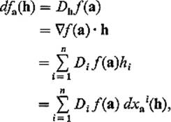
so the linear functions dfa and ![]() are equal. If we delete the subscript a, and write ∂f/∂xi for Di f(a), we obtain the classical formula
are equal. If we delete the subscript a, and write ∂f/∂xi for Di f(a), we obtain the classical formula
![]()
The mapping a → dfa, which associates with each point ![]() the linear function dfa :
the linear function dfa : ![]() n →
n → ![]() , is called a differential form, and Eq. (11) is the historical reason for this terminology. In Chapter V we shall discuss differential forms in detail.
, is called a differential form, and Eq. (11) is the historical reason for this terminology. In Chapter V we shall discuss differential forms in detail.
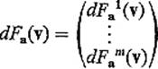
We now apply Theorem 2.2 to finish the computation of the derivative matrix F′(a). First we need the following lemma on “componentwise differentiation.”
Lemma 2.3 The mapping F: ![]() n →
n → ![]() m is differentiable at a if and only if each of its component functions F1, . . . , Fm is, and
m is differentiable at a if and only if each of its component functions F1, . . . , Fm is, and
![]()
(Here we have labeled the component functions with superscripts, rather than subscripts as usual, merely to avoid double subscripts.)
This lemma follows immediately from a componentwise reading of the vector equation (4).
Theorem 2.4 If F: ![]() n →
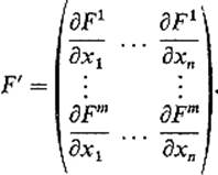
n → ![]() m is differentiable at a, then the matrix F′(a) of dFa is
m is differentiable at a, then the matrix F′(a) of dFa is
![]()
[That is, Dj Fi(a) is the element in the ith row and jth column of F′(a).]
PROOF
 (by Lemma 2.3)
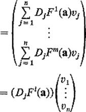 (by Theorem 2.2);
by the definition of matrix multiplication.
![]()
Finally we formulate a sufficient condition for differentiability. The mapping F: ![]() n →
n → ![]() m is said to be continuously differentiable at a if the partial derivatives D1 F, . . . , Dn F all exist at each point of some open set containing a, and are continuous at a.
m is said to be continuously differentiable at a if the partial derivatives D1 F, . . . , Dn F all exist at each point of some open set containing a, and are continuous at a.
Theorem 2.5 If F is continuously differentiable at a, then F is differentiable at a.
PROOF By (see Lemma 2.3), it suffices to consider a continuously differentiable real-valued function f: ![]() n →
n → ![]() . Given h = (h1, . . . , hn), let h0 = 0, hi = (h1, . . . , hi, 0, . . . , 0), i = 1, . . . , n (Fig. 2.9). Then
. Given h = (h1, . . . , hn), let h0 = 0, hi = (h1, . . . , hi, 0, . . . , 0), i = 1, . . . , n (Fig. 2.9). Then
![]()
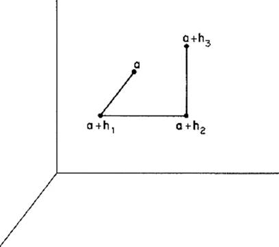
Figure 2.9
The single-variable mean value theorem gives
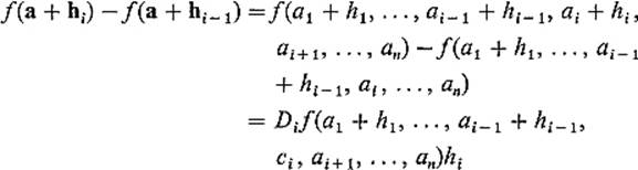
for some ![]() , since Dif is the derivative of the function
, since Dif is the derivative of the function
![]()
Thus f(a + hi) − f(a + hi−1) = hi Dif(bi) for some point bi which approaches a as h → 0. Consequently
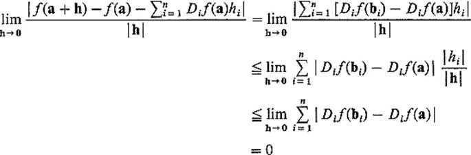
as desired, since each bi → a as h → 0, and each Dif is continuous at a.
![]()
Let us now summarize what has thus far been said about differentiability for functions of several variables, and in particular point out that the rather complicated concept of differentiability, as defined by Eq. (4), has now been justified.
For the importance of directional derivatives (rates of change) is obvious enough and, if a mapping is differentiable, then Theorem 2.2 gives a pleasant expression for its directional derivatives in terms of its partial derivatives, which are comparatively easy to compute; Theorem 2.4 similarly describes the derivative matrix. Finally Theorem 2.5 provides an effective test for the differentiability of a function in terms of its partial derivatives, thereby eliminating (in most cases) the necessity of verifying that it satisfies the definition of differentiability. In short, every continuously differentiable function is differentiable, and every differentiable function has directional derivatives; in general, neither of these implications may be reversed (see Example 4 and Exercise 2.5).
We began this section with a general discussion of tangent planes, which served to motivate the definition of differentiability. It is appropriate to conclude with an example in which our results are applied to actually compute a tangent plane.
Example 6 Let F: ![]() 2 →
2 → ![]() 4 be defined by
4 be defined by
![]()
Then F is obviously continuously differentiable, and therefore differentiable (Theorem 2.5). Let a = (1, 2), and suppose we want to determine the tangent plane to the image S of F at the point F(a) = (2, 1, 2, 3). By Theorem 2.4, the matrix of the linear mapping dFa : ![]() 2 →
2 → ![]() 4 is the 4 × 2 matrix
4 is the 4 × 2 matrix
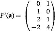
The image ![]() a of dFa is that subspace of
a of dFa is that subspace of ![]() 4 which is generated by the column vectors b1 = (0, 1, 2, −2) and b2 = (1, 0, 1, 4) of F′(a) (see Theorem I.5.2). Since b1 and b2 are linearly independent,
4 which is generated by the column vectors b1 = (0, 1, 2, −2) and b2 = (1, 0, 1, 4) of F′(a) (see Theorem I.5.2). Since b1 and b2 are linearly independent, ![]() a is 2-dimensional, and so is its orthogonal complement (Theorem I.3.4). In order to write
a is 2-dimensional, and so is its orthogonal complement (Theorem I.3.4). In order to write ![]() a in the form Ax = 0, we therefore need to find two linearly independent vectors a1 and a2 which are orthogonal to both b1 and b2; they will then be the row vectors of the matrix A. Two such vectors a1 and a2 are easily found by solving the equations
a in the form Ax = 0, we therefore need to find two linearly independent vectors a1 and a2 which are orthogonal to both b1 and b2; they will then be the row vectors of the matrix A. Two such vectors a1 and a2 are easily found by solving the equations
![]()
for example, a1 = (5, 0, −1, −1) and a2 = (0, 10, −4, 1).
The desired tangent plane T to S at the point F(a) = (2, 1, 2, 3) is now the parallel translate of ![]() a to F(a). That is, T is the set of all points
a to F(a). That is, T is the set of all points ![]() such that A(x − F(a)) = 0,
such that A(x − F(a)) = 0,
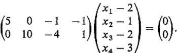
Upon simplification, we obtain the two equations
![]()
The solution set of each of these equations is a 3-dimensional hyperplane in ![]() 4; the intersection of these two hyperplanes is the desired (2-dimensional) tangent plane T.
4; the intersection of these two hyperplanes is the desired (2-dimensional) tangent plane T.
Exercises
2.1If F: ![]() n →
n → ![]() m is differentiable at a, show that F is continuous at a. Hint: Let
m is differentiable at a, show that F is continuous at a. Hint: Let
![]()
Then
![]()
2.2If p : ![]() 2 →
2 → ![]() is defined by p(x, y) = xy, show that p is differentiable everywhere with dp(a, b) (x, y) = bx + ay. Hint: Let L(x, y) = bx + ay, a = (a, b), h = (h, k). Then show that p(a + h) −p(a) − L(h) = hk. But
is defined by p(x, y) = xy, show that p is differentiable everywhere with dp(a, b) (x, y) = bx + ay. Hint: Let L(x, y) = bx + ay, a = (a, b), h = (h, k). Then show that p(a + h) −p(a) − L(h) = hk. But ![]() because
because ![]() .
.
2.3If f: ![]() 2 →
2 → ![]() is defined by f(x, y) = xy2/(x2 + y2) unless x = y = 0, and f(0, 0) = 0, show that Dvf(0, 0) exists for all v, but f is not differentiable at (0, 0). Hint: Note first that f(tv) = tf(v) for all
is defined by f(x, y) = xy2/(x2 + y2) unless x = y = 0, and f(0, 0) = 0, show that Dvf(0, 0) exists for all v, but f is not differentiable at (0, 0). Hint: Note first that f(tv) = tf(v) for all ![]() and
and ![]() . Then show that Dvf(0, 0) = f(v) for all v. Hence D1f(0, 0) = D2f(0, 0) = 0 but
. Then show that Dvf(0, 0) = f(v) for all v. Hence D1f(0, 0) = D2f(0, 0) = 0 but ![]() .
.
2.4Do the same as in the previous problem with the function f: ![]() 2 →
2 → ![]() defined by f(x, y) = (x1/3 + y1/3)3.
defined by f(x, y) = (x1/3 + y1/3)3.
2.5Let f : ![]() 2 →
2 → ![]() be defined by f(x, y) = x3 sin (1/x) + y2 for x ≠ 0, and f(0, y) = y2.
be defined by f(x, y) = x3 sin (1/x) + y2 for x ≠ 0, and f(0, y) = y2.
(a)Show that f is continuous at (0, 0).
(b) Find the partial derivatives of f at (0, 0).
(c) Show that f is differentiable at (0, 0).
(d) Show that D1 f is not continuous at (0, 0).
2.6Use the approximation ![]() fa ≈ dfa to estimate the value of
fa ≈ dfa to estimate the value of
(a)[(3.02)2 + (1.97)2 + (5.98)2],
(b)![]() .
.
2.7As in Exercise 1.3, a potential function for the vector field F : ![]() n →
n → ![]() n is a differentiable function V :
n is a differentiable function V : ![]() n →
n → ![]() such that F = −
such that F = −![]() V. Find a potential function for the vector field F defined for all x ≠ 0 by the formula
V. Find a potential function for the vector field F defined for all x ≠ 0 by the formula
(a)F(x) = rnx, where r = ![]() x
x![]() . Treat separately the cases n = 2 and n ≠ 2.
. Treat separately the cases n = 2 and n ≠ 2.
(b)F(x) = [g′(r)/r]x, where g is a differentiable function of one variable.
2.8Let f : ![]() n →
n → ![]() be differentiable. If f(0) = 0 and f(tx) = tf(x) for all
be differentiable. If f(0) = 0 and f(tx) = tf(x) for all ![]() and
and ![]() , prove that f(x) =
, prove that f(x) = ![]() f(0)·x for all
f(0)·x for all ![]() . In particular f is linear. Consequently any homogeneous function g :
. In particular f is linear. Consequently any homogeneous function g : ![]() n →
n → ![]() [meaning that g(tx) = tg(x)], which is not linear, must fail to be differentiable at the origin, although it has directional derivatives there (why?).
[meaning that g(tx) = tg(x)], which is not linear, must fail to be differentiable at the origin, although it has directional derivatives there (why?).
2.9If f : ![]() n →
n → ![]() m and g :
m and g : ![]() n →
n → ![]() k are both differentiable at
k are both differentiable at ![]() , prove directly from the definition that the mapping h :
, prove directly from the definition that the mapping h : ![]() n →
n → ![]() m+k, defined by h(x) = (f(x), g(x)), is differentiable at a.
m+k, defined by h(x) = (f(x), g(x)), is differentiable at a.
2.10Let the mapping F : ![]() 2 →
2 → ![]() 2 be defined by F(x1, x2) = (sin(x1 − x2), cos(x1 + x2)). Find the linear equations of the tangent plane in
2 be defined by F(x1, x2) = (sin(x1 − x2), cos(x1 + x2)). Find the linear equations of the tangent plane in ![]() 4 to the graph of F at the point (π/4, π/4, 0, 0).
4 to the graph of F at the point (π/4, π/4, 0, 0).
2.11Let f : ![]() 2uv →
2uv → ![]() 3xyz be the differentiable mapping defined by
3xyz be the differentiable mapping defined by
![]()
Let ![]() and
and ![]() . Given a unit vector u = (u, v), let
. Given a unit vector u = (u, v), let ![]() u :
u : ![]() →
→ ![]() 2 be the straight line through p, and ψu :
2 be the straight line through p, and ψu : ![]() →
→ ![]() 3 the curve through q, defined by
3 the curve through q, defined by ![]() u(t) = p + tu, ψu(t) = f(
u(t) = p + tu, ψu(t) = f(![]() u(t)), respectively. Then
u(t)), respectively. Then
![]()
by the definition of the directional derivative.
(a)For what unit vector(s) u is the speed ![]() ψu′(0)
ψu′(0)![]() maximal?
maximal?
(b)Suppose that g:![]() 3 →
3 → ![]() is a differentiable function such that
is a differentiable function such that ![]() g(q) = (1, 1, −1), and define
g(q) = (1, 1, −1), and define
![]()
Assuming the chain rule result that
![]()
find the unit vector u that maximizes hu′(0).
(c)Write the equation of the tangent plane to the image surface of f at the point f(1, 1) = (1, 0, 2).