Advanced Calculus of Several Variables (1973)

Part III. Successive Approximations and Implicit Functions

Chapter 3. THE INVERSE AND IMPLICIT MAPPING THEOREMS

The simplest cases of the inverse and implicit mapping theorems were discussed in Section 1. Theorem 1.3 dealt with the problem of solving an equation of the form f(x) = y for x as a function of y, while Theorem 1.4 dealt with the problem of solving an equation of the form G(x, y) = 0 for y as a function of x. In each case we defined a sequence of successive approximations which, under appropriate conditions, converged to a solution.

In this section we establish the analogous higher-dimensional results. Both the statements of the theorems and their proofs will be direct generalizations of those in Section 1. In particular we will employ the method of successive approximations by means of the contraction mapping theorem.

The definition of a contraction mapping in ⁿ is the same as on the line. Given a subset C of ⁿ, the mapping φ : C → C is called a contraction mapping with contraction constant k if

for all . The contraction mapping theorem asserts that, if the set C is closed and bounded, and k < 1, then φ has a unique fixed point such that φ(x_*) = x_*.

Theorem 3.1 Let φ : C → C be a contraction mapping with contraction constant k < 1, and with C being a closed and bounded subset of ⁿ. Then φ has a unique fixed point x_*. Moreover, given , the sequence defined inductively by

converges to x_*. In particular,

The proof given in see Section 1 for the case n = 1 generalizes immediately, with no essential change in the details. We leave it to the reader to check that the only property of the closed interval , that was used in the proof of Theorem 1.1, is the fact that every Cauchy sequence of points of [a, b] converges to a point of [a, b]. But every closed and bounded set has this property (the Appendix).

The inverse mapping theorem asserts that the mapping f : ⁿ → ⁿ is locally invertible in a neighborhood of the point if its differential df_a : ⁿ → ⁿ at a is invertible. This means that, if the linear mapping df_a : ⁿ→ ⁿ is one-to-one (and hence onto), then there exists a neighborhood U of a which f maps one-to-one onto some neighborhood V of b = f(a), with the inverse mapping g : V → U also being . Equivalently, if the linear equations

have a unique solution for each , then there exist neighborhoods U of a and V of b = f(a), such that the equations

have a unique solution for each . Here we are writing f¹, . . . , fⁿ for the component functions of f : ⁿ → ⁿ.

It is easy to see that the invertibility of df_a is a necessary condition for the local invertibility of f near a. For if U, V, and g are as above, then the compositions g f and f g are equal to the identity mapping on U and V, respectively. Consequently the chain rule implies that

This obviously means that df_a is invertible with . Equivalently, the derivative matrix f′(a) must be invertible with f′(a)⁻¹ = g′(b). But the matrix f′(a) is invertible if and only if its determinant is nonzero. So a necessary condition for the local invertibility of f near f′(a) is that f′(a) ≠ 0.

The following example shows that local invertibility is the most that can be hoped for. That is, f may be on the open set G with f′(a) ≠ 0 for each a ∈ G, without f being one-to-one on G.

Example 1 Consider the mapping f : ² → ² defined by

Since cos² θ − sin² θ = cos 2θ and 2 sin θ cos θ = sin 2θ, we see that in polar coordinates f is described by

From this it follows that f maps the circle of radius r twice around the circle of radius r². In particular, f maps both of the points (r cos θ, r sin θ) and (r cos (θ + π), r sin(θ + π)) to the same point (r² cos 2θ, r² sin 2θ). Thus f maps the open set ² − 0 “two-to-one” onto itself. However, f′(x, y) = 4(x² + y²), so f′(x, y) is invertible at each point of ² − 0.

We now begin with the proof of the inverse mapping theorem. It will be convenient for us to start with the special case in which the point a is the origin, with f(0) = 0 and f′(0) = I (the n × n identity matrix). This is the following substantial lemma; it contains some additional information that will be useful in Chapter IV (in connection with changes of variables in multiple integrals). Given ε > 0, note that, since f is with df₀ = I, there exists r > 0 such that df_x − I < ε for all points (the cube of radius r centered at C_r).

Lemma 3.2 Let f : ⁿ → ⁿ be a mapping such that f(0) = 0 and df₀ = I. Suppose also that

for all . Then

Moreover, if V = int C_{(1 − ε)r} and , then f : U → V is a one-to-one onto mapping, and the inverse mapping g : V → U is differentiable at 0.

Finally, the local inverse mapping g : V → U is the limit of the sequence of successive approximations defined inductively on V by

for y ∈ V.

PROOF We have already shown that (Corollary 2.7), and it follows from the proof of Corollary 2.8 that f is one-to-one on C_r—the cube C_r satisfies the conditions specified in the proof of Corollary 2.7. Alternatively, we can apply Corollary 2.6 with λ = df₀ = I to see that

if . From this inequality it follows that

The left-hand inequality shows that f is one-to-one on C_r, while the right-hand one (with y = 0) shows that .

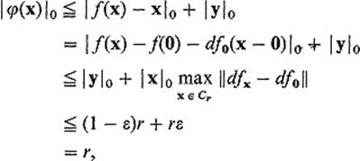
So it remains to show that f(C_r) contains the smaller cube C_{(1 − ε)r}. We will apply the contraction mapping theorem to prove this. Given , define φ : ⁿ → ⁿ by

We want to show that φ is a contraction mapping of C_r; its unique fixed point will then be the desired point such that f(x) = y.

To see that φ maps C_r into itself, we apply Corollary 2.6:

so if , then also. Note here that, if , then φ(x)₀ < r, so .

To see that φ : C_r → C_r is a contraction mapping, we need only note that

by (1).

Thus φ : C_r → C_r is indeed a contraction mapping, with contraction constant ε < 1, and therefore has a unique fixed point x such that f(x) = y. We have noted that φ maps C_r into int C_r if . Hence in this case the fixed point x lies in int C_r. Therefore, if , then U and V are open neighborhoods of 0 such that f maps U one-to-one onto V.

The fact that the fixed point x = g(y) is the limit of the sequence defined inductively by

follows immediately from the contraction mapping theorem (3.1).

So it remains only to show that g : V → U is differentiable at 0, where g(0) = 0. It suffices to show that

this will prove that g is differentiable at 0 with dg₀ = I. To verify (3), we apply (1) with y = 0, x = g(h), h = f(x), obtaining

We then apply the left-hand inequality of (2) with y = 0, obtaining

This follows from the fact that

Since f is at 0 with df₀ = I, we can make ε > 0 as small as we like, simply by restricting our attention to a sufficiently small (new) cube centered at 0. Hence (4) implies (3).

We now apply this lemma to establish the general inverse mapping theorem. It provides both the existence of a local inverse g under the condition f′(a) ≠ 0, and also an explicit sequence of successive approximations to g. The definition of this sequence can be motivated precisely as in the 1-dimensional case (preceding the statement of Theorem 1.3).

Theorem 3.3 Suppose that the mapping f : ⁿ → ⁿ is in a neighborhood W of the point a, with the matrix f′(a) being nonsingular. Then f is locally invertible—there exist neighborhoods of a and V of b = f(a), and a one-to-one mapping g : V → W such that

and

In particular, the local inverse g is the limit of the sequence of successive approximations defined inductively by

for y ∈ V.

PROOF We first “alter” the mapping f so as to make it satisfy the hypotheses of Lemma 3.2. Let τ_a and τ_b be the translations of ⁿ defined by

and let T = df_a : ⁿ → ⁿ. Then define : ⁿ → ⁿ by

The relationship between f and is exhibited by the following diagram:

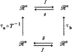
The assertion of Eq. (6) is that the same result is obtained by following the arrows around in either direction.

Note the (0) = 0. Since the differentials of τ_a and τ_b are both the identity mapping I of ⁿ, an application of the chain rule yields

Since is in a neighborhood of 0, we have

on a sufficiently small cube centered at 0. Therefore Lemma 3.2 applies to give neighborhoods and of 0, and a one-to-one mapping of onto , differentiable at 0, such that the mappings

are inverses of each other. Moreover Lemma 3.2 gives a sequence of successive approximations to , defined inductively by

for .

We let U = τ_a T⁻¹(), V = τ_b(), and define g : V → U by

(Now look at g and in the above diagram.) The facts, that is a local inverse to , and that the mappings τ_a T⁻¹ and τ_b are one-to-one, imply that g : V → U is the desired local inverse to f : U → V. The fact that is differentiable at 0 implies that g is differentiable at b = τ_b(0).

We obtain the sequence of successive approximations to g from the sequence of successive approximations to , by defining

for y ∈ V (replacing g by g_k and by _k in the above diagram).

To verify that the sequence may be defined inductively as in (5), note first that

Now start with the inductive relation

Substituting from (6) and (7), we obtain

Applying τ_a T⁻¹ to both sides of this equation, we obtain the desired inductive relation

It remains only to show that g : V → U is a mapping; at the moment we know only that g is differentiable at the point b = f(a). However what we have already proved can be applied at each point of U, so it follows that g is differentiable at each point of V.

To see that g is continuously ifferentiable on V, we note that, since

the chain rule gives

for each y ∈ V. Now f′(g(y)) is a continuous (matrix-valued) mapping, because f is by hypothesis, and the mapping g is continuous because it is differentiable (Exercise II.2.1). In addition it is clear from the formula for the inverse of a non-singular matrix (Theorem I.6.3) hat the entries of an inverse matrix A⁻¹ are continuous functions of those of A. These facts imply that the entries of the matrix g′(y) = [f′(g(y))]⁻¹ are continuous functions of y, so g is .

This last argument can be rephrased as follows. We can write g′: V → _nn, where _nn is the space of n × n matrices, as the composition

where (A) = A⁻¹ on the set of invertible n × n matrices (an open subset of _nn). is continuous by the above remark, and f′: U → _nn is continuous because f s , so we have expressed g′ as a composition of continuous mappings. Thus g′ is continuous, so g is by Proposition 2.4.

The power of the inverse mapping theorem stems partly from the fact that the condition det f′(a) ≠ 0 implies the invertibility of the mapping f in a neighborhood of a, even when it is difficult or impossible to find the local inverse mapping g explicitly. However Eqs. (5) enable us to approximate g rbitrarily closely [near b = f(a)].

Example 2 Suppose the mapping is defined by the equations

Let a = (1, −2), so b = f(a) = (2, −1). The derivative matrix is

so f′(a) is the identity matrix with determinant 1. Therefore f is invertible near a = (1, −2). That is, the above equations can be solved for u and v as functions of x and y, (u, v) = g(x, y), if the point (x, y) is sufficiently close to b = (2, −1). According to Eqs. (5), the sequence of successive approximations is defined inductively by

Writing g_k(x, y) = (u_k, v_k), we have

The first several approximations are

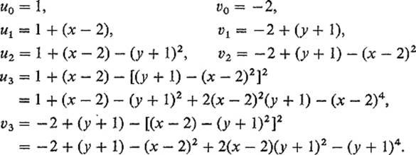
It appears that we are generating Taylor polynomials for the component functions of g in powers of (x − 2) and (y + 1). This is true, but we will not verify it.

The inverse mapping theorem tells when we can, in principle, solve the equation x = f(y), or equivalently x − f(y) = 0, for y as a function of x. The implicit mapping theorem deals with the problem of solving the general equation G(x, y) = 0, for y as a function of x. Although the latter equation may appear considerably more general, we will find that its solution reduces quite easily to the special case considered in the inverse mapping theorem.

In order for us to reasonably expect a unique solution of G(x, y) = 0, there should be the same number of equations as unknowns. So if , then G should be a mapping from ^{m + n} to ⁿ. Writing out components of the vector equation G(x, y) = 0, we obtain

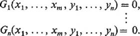
We want to discuss the solution of this system of equations for y₁, . . . , y_n in terms of x₁, . . . , x_m.

In order to investigate this problem we need the notion of partial differential linear mappings. Given a mapping G : ^{m + n} → ^k wihch is differentiable at the point , the partial differentials of G are the linear mappings d_x G_p : ^m → ^k and d_y G_p: ⁿ → ^k defined by

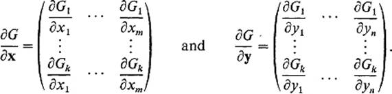
respectively. The matrices of these partial differential linear mappings are called the partial derivatives of G with respect to x and y, respectively. These partial derivative matrices are denoted by

respectively. It should be clear from the definitions that D₁G(a, b) consists of the first m columns of G′(a, b), while D₂ G(a, b) consists of the last n columns. Thus

Suppose now that and are both differentiable functions of and y = β(t), and define φ : ¹ → ^k by

Then a routine application of the chain rule gives the expected result

or

in more detail. We leave this computation to the exercises (Exercise 3.16). Note that D₁G is a k × m matrix and α′ is an m × l matrix, while D₂ G is a k × n matrix and β′ is an n × l matrix, so Eq. (8) at least makes sense.

Suppose now that the function G : ^{m + n} → ⁿ is differentiable in a neighborhood of the point where G(a, b) = 0. Suppose also that the equation G(x, y) = 0 implicitly defines a differentiable function y = h(x) for x near a, that is, h is a differentiable mapping of a neighborhood of a into ⁿ, with

We can then compute the derivative h′(x) by differentiating the equation G(x, h(x)) = 0. Applying Eq. (8) above with x = t, α(x) = x, we obtain

If the n × n matrix D₂ G(x, y) is nonsingular, it follows that

In particular, it appears that the nonvanishing of the so-called Jacobian determinant

at (a, b) is a necessary condition for us to be able to solve for h′(a). The implicit mapping theorem asserts that, if G is in a neighborhood of (a, b), then this condition is sufficient for the existence of the implicitly defined mapping h.

Given G : ^{m + n} → ⁿ and h : U → ⁿ, where , we will say that y = h(x) solves the equation G(x, y)) = 0 in a neighborhood W of (a, b) if the graph of f agrees in W with the zero set of G. That is, if (x,y)∈ W and x ∈ U, then

Note the almost verbatim analogy between the following general implicit mapping theorem and the case m = n = 1 considered in Section 1.

Theorem 3.4 Let the mapping G : ^{m + n} → ⁿ be in a neighborhood of the point (a, b) where G(a, b) = 0. If the partial derivative matrix D₂ G(a, b) is nonsingular, then there exists a neighborhood U of a in ^m, a neighborhood W of (a, b) in ^{m + n}, and a mapping h : U → ⁿ, such that y = h(x) solves the equation G(x, y) = 0 in W.

In particular, the implicitly defined mapping h is the limit of the sequence of successive approximations defined inductively by

for x ∈ U.

PROOF We want to apply the inverse mapping theorem to the mapping f : ^{m + n} → ^{m + n} defined by

for which f(x, y) = (x, 0) if and only if G(x, y) = 0. Note that f is in a neighborhood of the point (a, b) where f(a, b) = (a, 0). In order to apply the inverse mapping theorem in a neighborhood of (a, b), we must first show that the matrix f′(a, b) is nonsingular.

It is clear that

where I denotes the m × m identity matrix, and 0 denotes the m × n zero matrix. Consequently

if . In order to prove that f′(a, b) is nonsingular, it suffices to show that df_{(a, b)} is one-to-one (why?), that is, that df_{(a, b)}(r, s) = (0, 0) implies (r, s) = (0, 0). But this follows immediately from the above expression for df_{(a, b)}(r, s) and the hypothesis that D₂ G(a, b) is nonsingular, so d_y G_{(a, b)}(s) = 0 implies s = 0.

We can therefore apply the inverse mapping theorem to obtain neighborhoods W of (a, b) and V of (a, 0), and a inverse g : V → W of f : W → V, such that g(a, 0) = (a, b). Let U be the neighborhood of defined by

identifying ^m with (see Fig. 3.8).

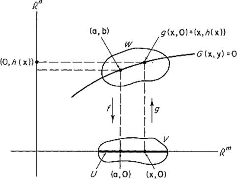
Figure 3.8

Since f(x, y) = 0 if and only if G(x, y) = 0, it is clear that g maps the set one-to-one onto the intersection with W of the zero set G(x, y) = 0. If we now define the mapping h : U → ⁿ by

it follows that y = h(x) solves the equation G(x, y) = 0 in W.

It remains only to define the sequence of successive approximations to h. The inverse mapping theorem provides us with a sequence of successive approximations to g, defined inductively by

We define h_k : U → ⁿ by

Then the fact, that the sequence converges to g on V, implies that the sequence converges to h on U.

Since g₀(x, y) ≡ (a, b), we see that h₀(x) ≡ b. Finally

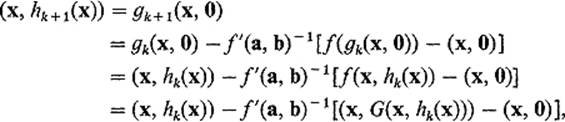
so

Taking second components of this equation, we obtain

as desired.

Example 3 Suppose we want to solve the equations

for y and z as functions of x in a neighborhood of (− 1, 1, 0). We define G : ³ → ² by

Since

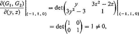
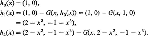
the implicit mapping theorem assures us that the above equations do implicitly define y and z as functions of x, for x near − 1. The successive approximations for h(x) = (y(x), z(x)) begin as follows:

Example 4 Let G : ² × ² = ⁴ → ² be defined by

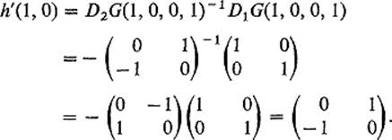
where x = (x₁, x₂) and y = (y₁, y₂), and note that G(1, 0, 0, 1) = (0, 0). Since

is nonsingular, the equation G(x, y) = 0 defines y implicitly as a function of x, y = h(x) for x near (1, 0). Suppose we only want to compute the derivative matrix h′(1, 0). Then from Eq. (9) we obtain

Note that, writing Eq. (9) for this example with Jacobian determinants instead of derivative matrices, we obtain the chain rule type formula

or

The partial derivatives of an implicitly defined function can be calculated using the chain rule and Cramer's rule for solving linear equations. The following example illustrates this procedure.

Example 5 Let G₁, G₂ : ⁵ → be functions, with G₁(a) = G₂(a) = 0 and

at the point . Then the two equations

implicitly define u and v as functions of x, y, z:

Upon differentiation of the equations

with respect to x, we obtain

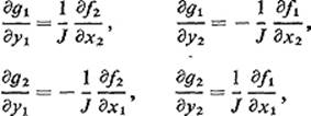
Solving these two linear equations for ∂f/∂x and ∂g/∂x, we obtain

Similar formulas hold for ∂f/∂y, ∂g/∂y, ∂f/∂z, ∂g/∂z (see Exercise 3.18).

Exercises

3.1Show that f(x, y) = (x/(x² + y²), y/(x² + y²)) is locally invertible in a neighborhood of every point except the origin. Compute f⁻¹ explicitly.

3.2Show that the following mappings from ² to itself are everywhere locally invertible.

(a)f(x, y) = (e^x + e^y, e^x − e^y).

(b)g(x, y) = (e^x cos y, e^x sin y).

3.3Consider the mapping f : ³ → ³ defined by f(x, y, z) = (x, y³, z⁵). Note that f has a (global) inverse g, despite the fact that the matrix f′(0) is singular. What does this imply about the differentiability of g at 0?

3.4Show that the mapping , defined by u = x + e^y, v = y + e^z, w = z + e^x, is everywhere locally invertible.

3.5Show that the equations

implicitly define z near − 1, as a function of (x, y) near (1, 1).

3.6Can the surface whose equation is

be represented in the form z = f(x, y) near (0, 2, 1)?

3.7Decide whether it is possible to solve the equations

for (u, v) near (1, 1) as a function of (x, y, z) near (1, 1, 1).

3.8The point (1, −1, 1) lies on the surfaces

Show that, in a neighborhood of this point, the curve of intersection of the surfaces can be described by a pair of equations of the form y = f(x), z = g(x).

3.9Determine an approximate solution of the equation

for z near 2, as a function of (x, y) near (1, −1).

3.10If the equations f(x, y, z) = 0, g(x, y, z) = 0 can be solved for y and z as differentiable functions of x, show that

where J = ∂(f, g)/∂(y, z).

3.11If the equations f(x, y, u, v) = 0, g(x, y, u, v) = 0 can be solved for u and v as differentiable functions of x and y, compute their first partial derivatives.

3.12Suppose that the equation f(x, y, z) = 0 can be solved for each of the three variables x, y, z as a differentiable function of the other two. Then prove that

Verify this in the case of the ideal gas equation pv = RT (where p, v, T are the variables and R is a constant).

3.13Let and be inverse functions. Show that

where J = ∂(f₁, f₂)/∂(x₁, x₂).

3.14Let and be inverse functions. Show that

and obtain similar formulas for the other derivatives of component functions of g.

3.15Verify the statement of the implicit mapping theorem given in Section II.5.

3.16Verify Eq. (8) in this section.

3.17Suppose that the pressure p, volume v, temperature T, and internal energy u of a gas satisfy the equations

and that these two equations can be solved for any two of the four variables as functions of the other two. Then the symbol ∂u/∂T, for example, is ambiguous. We denote by (∂u/∂T)_p the partial derivative of u with respect to T, with u and v considered as functions of p and T, and by (∂u/∂T)_vthe partial derivative of u, with u and p considered as functions of v and T. With this notation, apply the results of Exercise 3.11 to show that

3.18If y₁, . . . , y_n are implicitly defined as differentiable functions of x₁, . . . , x_m by the equations

show, by generalizing the method of Example 5, that

where