Advanced Calculus of Several Variables (1973)

Part I. Euclidean Space and Linear Mappings

Chapter 3. INNER PRODUCTS AND ORTHOGONALITY

In order to obtain the full geometric structure of ⁿ (including the concepts of distance, angles, and orthogonality), we must supply ⁿ with an inner product. An inner (scalar) product on the vector space V is a function V × V → , which associates with each pair (x, y) of vectors in V a real number x, y, and satisfies the following three conditions:

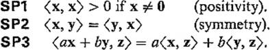
The third of these conditions is linearity in the first variable; symmetry then gives linearity in the second variable also. Thus an inner product on V is simply a positive, symmetric, bilinear function on V × V. Note that SP3 implies that 0, 0 = 0 (see Exercise 3.1).

The usual inner product on ⁿ is denoted by x · y and is defined by

where x = (x₁, . . . , x_n), y = (y₁, . . . , y_n). It should be clear that this definition satisfies conditions (SP1, SP2, SP3 above. There are many inner products on ⁿ see Example 2 below), but we shall use only the usual one.

Example 1Denote by the vector space of all continuous functions on the interval [a, b], and define

for any pair of functions It is obvious that this definition satisfies conditions SP2 and SP3. It also satisfies SP1, because if f(t₀) ≠ 0, then by continuity (f(t))² > 0 for all t in some neighborhood of t₀, so

Therefore we have an inner product on .

Example 2Let a, b, c be real numbers with a > 0, ac − b² > 0, so that the quadratic form q(x) = ax₁² + 2bx₁x₂ + cx₂² is positive-definite (see Section II.4). Then x, y = ax₁y₁ + bx₁y₂ + bx₂y₁ + cx₂y₂ defines an inner product on ² (why?). With a = c = 1, b = 0 we obtain the usual inner product on ².

An inner product on the vector space V yields a notion of the length or “size” of a vector , called its norm x. In general, a norm on the vector space V is a real-valued function x → x on V satisfying the following conditions:

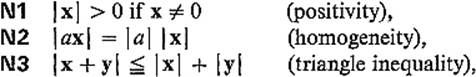
for all and . Note that N2 implies that 0 = 0.

The norm associated with the inner product , on V is defined by

It is clear that SP1–SP3 and this definition imply conditions N1 and N2, but the triangle inequality is not so obvious; it will be verified below.

The most commonly used norm on ⁿ is the Euclidean norm

which comes in the above way from the usual inner product on ⁿ. Other norms on ⁿ, not necessarily associated with inner products, are occasionally employed, but henceforth x will denote the Euclidean norm unless otherwise specified.

Example 3x = max {x₁, . . . , x_n}, the maximum of the absolute values of the coordinates of x, defines a norm on ⁿ (see Exercise 3.2).

Example 4x₁ = x₁ + x₂ + · · · + x_n defines still another norm on ⁿ (again see Exercise 3.2).

A norm on V provides a definition of the distance d(x, y) between any two points x and y of V:

Note that a distance function d defined in this way satisfies the following three conditions:

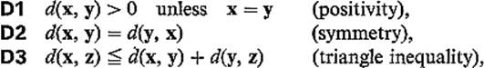
for any three points x, y, z. Conditions D1 and D2 follow immediately from N1 and N2, respectively, while

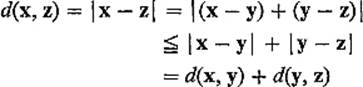
by N3. Figure 1.1 indicates why N3 (or D3) is referred to as the triangle inequality.

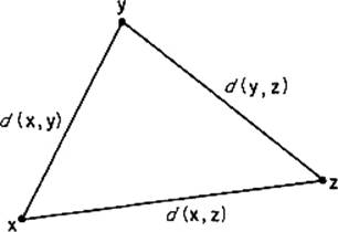
Figure 1.1

The distance function that comes in this way from the Euclidean norm is the familiar Euclidean distance function

Thus far we have seen that an inner product on the vector space V yields a norm on V, which in turn yields a distance function on V, except that we have not yet verified that the norm associated with a given inner product does indeed satisfy the triangle inequality. The triangle inequality will follow from the Cauchy–Schwarz inequality of the following theorem.

Theorem 3.1If , is an inner product on a vector space V, then

for all [where the norm is the one defined by (2)].

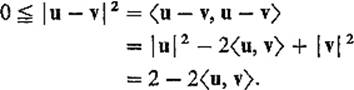
PROOFThe inequality is trivial if either x or y is zero, so assume neither is. If u = x/x and v = y/y, then u = v = 1. Hence

So that is or

Replacing x by −x, we obtain

also, so the inequality follows.

The Cauchy–Schwarz inequality is of fundamental importance. With the usual inner product in ⁿ, it takes the form

while in , with the inner product of Example 1, it becomes

PROOFOF THE TRIANGLE INEQUALITY Given note that

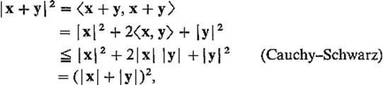
which implies that

Notice that, if x, y = 0, in which case x and y are perpendicular (see the definition below), then the second equality in the above proof gives

This is the famous theorem associated with the name of Pythagoras (Fig. 1.2).

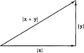
Figure 1.2

Recalling the formula x · y = x y cos θ for the usual inner product in ², we are motivated to define the angle (x, y) between the vectors by

Notice that this makes sense because by the Cauchy–Schwarz inequality. In particular we say that x and y are orthogonal (or perpendicular) if and only if x · y = 0, because then (x, y) = arccos π/2 = 0.

A set of nonzero vectors v₁, v₂, . . . in V is said to be an orthogonal set if

whenever i ≠ j. If in addition each v_i is a unit vector, v_i, v_i = 1, then the set is said to be orthonormal.

Example 5The standard basis vectors e₁, . . . , e_n form an orthonormal set in ⁿ.

Example 6The (infinite) set of functions

is orthogonal in (see Example 1 and Exercise 3.11). This fact is the basis for the theory of Fourier series.

The most important property of orthogonal sets is given by the following result.

Theorem 3.2Every finite orthogonal set of nonzero vectors is linearly independent.

PROOFSuppose that

Taking the inner product with v_i, we obtain

because v_i, v_i = 0 for i ≠ j if the vectors v₁, . . . , v_k are orthogonal. But v_i, v_i ≠ 0, so a_i = 0. Thus (3) implies a₁ = · · · = a_k = 0, so the orthogonal vectors v₁, . . . , v_k are linearly independent.

We now describe the important Gram–Schmidt orthogonalization process for constructing orthogonal bases. It is motivated by the following elementary construction. Given two linearly independent vectors v and w₁, we want to find a nonzero vector w₂ that lies in the subspace spanned by v and w₁, and is orthogonal to w₁. Figure 1.3 suggests that such a vector w₂ can be obtained by subtracting from v an appropriate multiple cw₁ of w₁. To determine c,

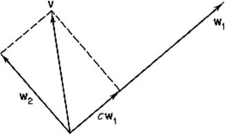
Figure 1.3

we simply solve the equation w₁, v − cw₁ = 0 for c = v, w₁/w₁, w₁. The desired vector is therefore

obtained by subtracting from v the “component of v parallel to w₁.” We immediately verify that w₂, w₁ = 0, while w₂ ≠ 0 because v and w₁ are linearly independent.

Theorem 3.3If V is a finite-dimensional vector space with an inner product, then V has an orthogonal basis.

In particular, every subspace of ⁿ has an orthogonal basis.

PROOFWe start with an arbitrary basis v₁, . . . , v_n for V. Let w₁ = v₁. Then, by the preceding construction, the nonzero vector

is orthogonal to w₁ and lies in the subspace generated by v₁ and v₂.

Suppose inductively that we have found an orthogonal basis w₁, . . . , w_k for the subspace of V that is generated by v₁, . . . , v_k. The idea is then to obtain w_k+1 by subtracting from v_k+1 its components parallel to each of the vectors w₁, . . . , w_k. That is, define

where c_i = v_k+1, w_i/w_i, w_i. Then w_k+1, w_i = v_k+1, w_i − c_iw_i, w_i = 0 for , and w_k+1 ≠ 0, because otherwise v_k+1 would be a linear combination of the vectors w₁, . . . , w_k, and therefore of the vectors v₁, . . . , v_k. It follows that the vectors w₁, . . . , w_k+1 form an orthogonal basis for the subspace of V that is generated by v₁, . . . , v_k+1.

After a finite number of such steps we obtain the desired orthogonal basis w₁, . . . , w_n for V.

It is the method of proof of Theorem 3.3 that is known as the Gram–Schmidt orthogonalization process, summarized by the equations

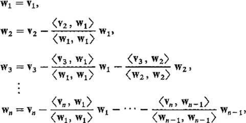
defining the orthogonal basis w₁, . . . , w_n in terms of the original basis v₁, . . . , v_n.

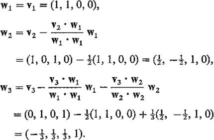
Example 7To find an orthogonal basis for the subspace V of ⁴ spanned by the vectors v₁ = (1, 1, 0, 0), v₂ = (1, 0, 1, 0), v₃ = (0, 1, 0, 1), we write

Example 8Let denote the vector space of polynomials in x, with inner product defined by

By applying the Gram–Schmidt orthogonalization process to the linearly independent elements 1, x, x², . . . , xⁿ, . . . , one obtains an infinite sequence , the first five elements of which are (see Exercise 3.12). Upon multiplying the polynomials {p_n(x)} by appropriate constants, one obtains the famous Legendre polynomials etc.

One reason for the importance of orthogonal bases is the ease with which a vector can be expressed as a linear combination of orthogonal basis vectors w₁, . . . , w_n for V. Writing

and taking the inner product with w_i, we immediately obtain

so

This is especially simple if w₁, . . . , w_n is an orthonormal basis for V:

Of course orthonormal basis vectors are easily obtained from orthogonal ones, simply by dividing by their lengths. In this case the coefficient v · w_i of w_i in (5) is sometimes called the Fourier coefficient of v with respect to w_i. This terminology is motivated by an analogy with Fourier series. The orthonormal functions in corresponding to the orthogonal functions of Example 6 are

Writing

one defines the Fourier coefficients of by

and

It can then be established, under appropriate conditions on f, that the infinite series

converges to f(x). This infinite series may be regarded as an infinite-dimensional analog of (5).

Given a subspace V of ⁿ, denote by V the set of all those vectors in ⁿ, each of which is orthogonal to every vector in V. Then it is easy to show that V is a subspace of ⁿ, called the orthogonal complement of V (Exercise 3.3). The significant fact about this situation is that the dimensions add up as they should.

Theorem 3.4If V is a subspace of ⁿ, then

PROOF By Theorem 3.3, there exists an orthonormal basis v₁, . . . , v_r for V, and an orthonormal basis w₁, . . . , w_s for V. Then the vectors v₁, . . . , v_r, w₁, . . . , w_s are orthornormal, and therefore linearly independent. So in order to conclude from Theorem 2.5 that r + s = n as desired, it suffices to show that these vectors generate ⁿ. Given , define

Then y · v_i = x · v_i − (x · v_i)(v_i · v_i) = 0 for each i = 1, . . . , r. Since y is orthogonal to each element of a basis for V, it follows easily that (Exercise 3.4). Therefore Eq. (5) above gives

This and (7) then yield

so the vectors v₁, . . . , v_r, w₁, . . . , w_s constitute a basis for ⁿ.

Example 9Consider the system

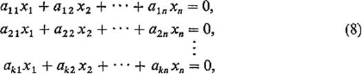
of homogeneous linear equations in x₁, . . . , x_n. If a_i = (a_i1, . . . , a_in), i = 1, . . . , k, then these equations can be rewritten as

Therefore the set S of all solutions of (8) is simply the set of all those vectors that are orthogonal to the vectors a₁, . . . , a_k. If V is the subspace of ⁿ generated by a₁, . . . , a_k, it follows that S = V (Exercise 3.4). If the vectors a₁, . . . , a_k are linearly independent, we can then conclude from Theorem 3.4 that dim S = n − k.

Exercises

3.1Conclude from condition SP3 that 0, 0 = 0.

3.2Verify that the functions defined in Examples 3 and 4 are norms on ⁿ.

3.3If V is a subspace of ⁿ, prove that V is also a subspace.

3.4If the vectors a₁, . . . , a_k generate the subspace V of ⁿ, and is orthogonal to each of these vectors, show that .

3.5Verify the “polarization identity”

3.6Let a₁, a₂, . . . , a_n be an orthonormal basis for ⁿ. If x = s₁a₁ + · · · + s_na_n and y = t₁a₁ + · · · + t_na_n, show that x · y = s₁t₁ + · · · + s_n t_n. That is, in computing x · y, one may replace the coordinates of x and y by their components relative to any orthonormal basis for ⁿ.

3.7Orthogonalize the basis (1, 0, 0, 1), (−1, 0, 2, 1), (0, 1, 2, 0), (0, 0, −1, 1) in ⁴.

3.8Orthogonalize the basis

in ⁿ.

3.9Find an orthogonal basis for the 3-dimensional subspace V of ⁴ that consists of all solutions of the equation x₁ + x₂ + x₃ − x₄ = 0. Hint: Orthogonalize the vectors v₁ = (1, 0, 0, 1), v₂ = (0, 1, 0, 1), v₃ = (0, 0, 1, 1).

3.10Consider the two equations

Let V be the set of all solutions of (*) and W the set of all solutions of both equations. Then W is a 2-dimensional subspace of the 3-dimensional subspace V of ⁴ (why?).

(a) Solve (*) and (**) to find a basis v₁, v₂ for W.

(b) Find by inspection a vector v₃ which is in V but not in W. Why is v₁, v₂, v₃ then a basis for V?

(c) Orthogonalize v₁, v₂, v₃ to obtain an orthogonal basis w₁, w₂, w₃ for V, with w₁ and w₂ in W.

(d) Normalize w₁, w₂, w₃ to obtain an orthonormal basis u₁, u₂, u₃ for V. Express v = (11, 3, 6, −11) as a linear combination of u₁, u₂, u₃.

(e) Find vectors and such that v = x + y.

3.11Show that the functions

are orthogonal in the inner product space of Example 1.

3.12Orthogonalize in the functions 1, x, x², x³, x⁴ to obtain the polynomials p₀(x), . . . , p₄(x) listed in Example 8.