Advanced Calculus of Several Variables (1973)

Part VI. The Calculus of Variations

Chapter 4. THE ISOPERIMETRIC PROBLEM

In this section we treat the so-called isoperimetric problem that was mentioned in the introduction to this chapter. Given functions f, g : ³ → , we wish to maximize or minimize the function

subject to the endpoint conditions ψ(a) = α, ψ(b) = β and the constraint

If, as in Section 3, we denote by M the hyperplane in consisting of all those functions ψ : [a, b] → such that ψ(a) = α and (b) = β, then our problem is to locate the local extrema of the function F on the set .

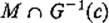The similarity between this problem and the constrained maximum–minimum problems of Section II.5 should be obvious—the only difference is that here the functions F and G are defined on the infinite-dimensional normed vector space , rather than on a finite-dimensional Euclidean space. So our method of attack will be to appropriately generalize the method of Lagrange multipliers so that it will apply in this context.

First let us recall Theorem II.5.5 in the following form. Let F, G : ⁿ → be functions such that G(0) = 0 and ∇G(0) ≠ 0. If F has a local maximum or local minimum at 0 subject to the constraint G(x) = 0, then there exists a number λ such that

Since the differentials dF₀, dG₀ : ⁿ → are given by

Eq. (3) can be rewritten

where Λ : → is the linear function defined by Λ(t) = λt.

Equation (4) presents the Lagrange multiplier method in a form which is suitable for generalization to normed vector spaces (where differentials are available, but gradient vectors are not). For the proof we will need the following elementary algebraic lemma.

Lemma 4.1 Let α and β be real-valued linear functions on the vector space E such that

Then there exists a linear function Λ : → such that α = Λ β. That is, the following diagram of linear functions “commutes.”

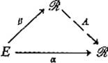
PROOF Given , pick such that β(x) = t, and define

In order to show that Λ is well defined, we must see that, if y is another element of E with β(y) = t, then α(x) = α(y). But if β(x) = β(y) = t, then so α(x − y) = 0, which immediately implies that α(x) = α(y).

If β(x) = s and β(y) = t, then

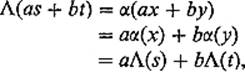
so Λ is linear.

The following theorem states the Lagrange multiplier method in the desired generality.

Theorem 4.2 Let F and G be real-valued functions on the complete normed vector space E, with G(0) = 0 and dG₀ ≠ 0 (so Im dG₀ = ). If F : E → has a local extremum at 0 subject to the constraint G(x) = 0, then there exists a linear function λ : → such that

Of course the statement, that “F has a local extremum at 0 subject to G(x) = 0,” means that the restriction FG⁻¹(0) has a local extremum at .

PROOF This will follow from Lemma 4.1, with α = dF₀ and β = dG₀, if we can prove that Ker dF₀ contains Ker dG₀. In order to do this, let us first assume the fact (to be established afterward) that, given , there exists a differentiable path γ : (−, ) → E whose image lies in G⁻¹(0), such that γ(0) = 0 and γ′(0) = v (see Fig. 6.6).

Then the composition h = F γ : (−, ) → has a local extremum at 0, so h′(0) = 0. The chain rule therefore gives

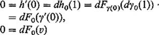
as desired.

We will use the implicit function theorem to verify the existence of the differentiable path γ used above. If X = Ker dG₀ then, since dG₀ : E → is continuous, X is a closed subspace of E, and is therefore complete (by Exercise 1.5). Choose such that dG₀(w) = 1, and denote by Y the closed subspace of E consisting of all scalar multiples of w; then Y is a “copy” of .

It is clear that . Also, if and , then

so . Therefore

with and . Thus E is the algebraic direct sum of the subspaces X and Y. Moreover, it is true (although we omit the proof) that the norm on E is equivalent to the product norm on X × Y, so we may write E = X × Y.

In order to apply the implicit function theorem, we need to know that

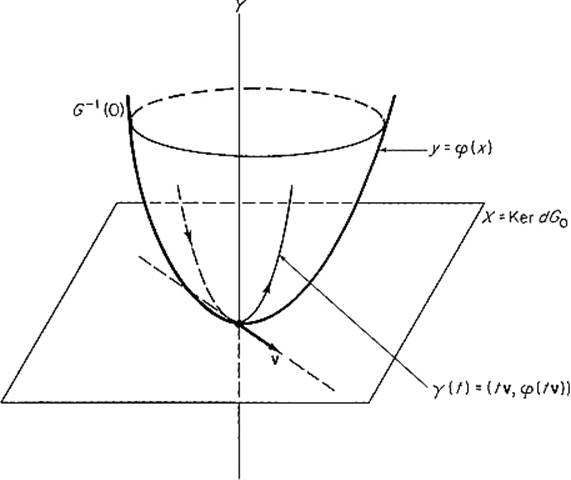
Figure 6.6

is an isomorphism. Since Y ≈ , we must merely show that d_y G₀ ≠ 0. But, given , we have

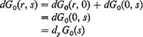
by Exercise 2.6, so the assumption that d_y G₀ = 0 would imply that dG₀ = 0, contrary to hypothesis.

Consequently the implicit function theorem provides a function φ : X → Y whose graph y = φ(x) in X × Y = E coincides with G⁻¹(0), inside some neighborhood of 0. If H(x) = G(x, φ(x)), then H(x) = 0 for x near 0, so

for all . It therefore follows that dφ₀ = 0, because d_y G₀ is an isomorphism.

Finally, given , define γ : → E by γ(t) = (tu, φ(tu)). Then γ(0) = 0 and 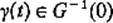for t sufficiently small, and

as desired.

We are now prepared to deal with the isoperimetric problem. Let f and g be real-valued functions on ³, and define the real-valued functions F and G on by

and

where . Assume that φ is a element of at which F has a local extremum on 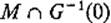, where M is the usual hyperplane in that is determined by the endpoint conditions (a) = α and (b) = β.

We have seen (in Section 3) that M is the translate (by any fixed element of M) of the subspace of consisting of these elements 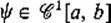such that (a) = (b) = 0. Let be the translation defined by

and note that T(0) = φ, while

is the identity mapping.

Now consider the real-valued functions F T and G T on . The fact that F has a local extremum on at φ implies that F T has a local extremum at 0 subject to the condition G T() = 0.

Let us assume that φ is not an extremal for G on M, that is, that

so d(G T)₀ ≠ 0. Then Theorem 4.2 applies to give a linear function Λ : → such that

Since dT₀ is the identity mapping on C₀¹[a, b], the chain rule gives

on . Writing Λ(t) = λt and applying the computation of Corollary 3.2 for the differentials dF_φ and dG_φ, we conclude that

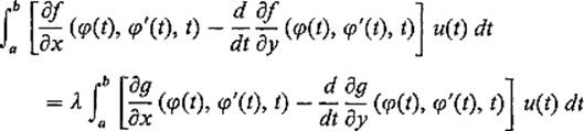
for all .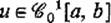

If h : ³ → is defined by

it follows that

for all . An application of Lemma 3.3 finally completes the proof of the following theorem.

Theorem 4.3 Let F and G be the real-valued functions on defined by (6) and (7), where f and g are functions on ³. Let be a function which is not an extremal for G. If F has a local extremum at φ subject to the conditions

then there exists a real number λ such that φ satisfies the Euler–Lagrange equation for the function h = f − λg, that is,

for all .

The following application of this theorem is the one which gave such constraint problems in the calculus of variations their customary name—isoperimetric problems.

Example Suppose φ : [a, b] → is that nonnegative function (if any) with φ(a) = φ(b) = 0 whose graph x = φ(t) has length L, such that the area under its graph is maximal. We want to prove that the graph x = φ(t) must be an arc of

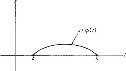
Figure 6.7

a circle (Fig. 6.7). If f(x, y, t) = x and , then φ maximizes the integral

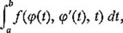
subject to the conditions

Since , the Euler-Lagrange equation (8) is

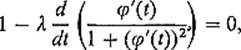
or

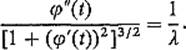
This last equation just says that the curvature of the curve t → (t, φ(t)) is the constant 1/λ. Its image must therefore be part of a circle.

The above discussion of the isoperimetric problem generalizes in a straightforward manner to the case in which there is more than one constraint. Given functions f, g₁, . . . , g_k: ³ → , we wish to minimize or maximize the function

subject to the endpoint conditions (a) = α, (b) = β and the constraints

Our problem then is to locate the local extrema of F on , where M is the usual hyperplane in and

The result, analogous to Theorem 4.3, is as follows.

Let be a function which is not an extremal for any linear combination of the functions G₁, . . . , G_k. If F has a local extremum at φ subject to the conditions

then there exist numbers λ₁, . . . , λ_k such that φ satisfies the Euler–Lagrange equation for the function

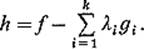
Inclusion of the complete details of the proof would be repetitious, so we simply outline the necessary alterations in the proof of Theorem 4.3.

First Lemma 4.1 and Theorem 4.2 are slightly generalized as follows. In Lemma 4.1 we take β to be a linear mapping from E to ^k with Im β = ^k, and in Theorem 4.2 we take G to be a mapping from E to ^k such that G(0) = 0 and Im dG₀ = ^k. The only other change is that, in the conclusion of each, Λ becomes a real-valued linear function on ^k. The proofs remain essentially the same.

We then apply the generalized Theorem 4.2 to the mappings and , defined by (9) and (10), in the same way that the original (Theorem 4.2) was applied (in the proof of Theorem 4.3) to the functions defined by (6) and (7). The only additional observation needed is that, if φ is not an extremal for any linear combination of the component functions G₁, . . . , G_k, then it follows easily that dG_φ maps TM_φ onto ^k. We then conclude as before that

for some linear function Λ : ^k → . Writing , we conclude that

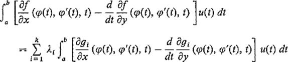
for all . An application of Lemma 3.3 then implies that φ satisfies the Euler–Lagrange equation for .

Exercises

4.1Consulting the discussion at the end of Section 3, generalize the isoperimetric problem to the vector-valued case as follows: Let f, g : ⁿ × ⁿ × → be given functions, and suppose φ : [a, b] → ⁿ is an extremal for

subject to the conditions (a) = α, (b) = β and

Then show under appropriate conditions that, for some number λ, the path φ satisfies the Euler–Lagrange equations

for the function h = f − λg.

4.2Let φ : [a, b] → ² be a closed curve in the plane, φ(a) = φ(b), and write φ(t) = (x(t), y(t)). Apply the result of the previous problem to show that, if φ maximizes the area integral

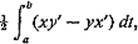
subject to

then the image of φ is a circle.

4.3With the notation and terminology of the previous problem, establish the following reciprocity relationship. The closed path φ is an extremal for the area integral, subject to the arclength integral being constant, if and only if φ is an extremal for the arclength integral subject to the area integral being constant. Conclude that, if φ has minimal length amongst curves enclosing a given area, then the image of φ is a circle.

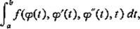
4.4Formulate (along the lines of Exercise 3.9) a necessary condition that φ : [a, b] → minimize

subject to

This is the isoperimetric problem with second derivatives.

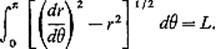
4.5Suppose that describes (in polar coordinates) a closed curve of length L that encloses maximal area. Show that it is a circle by maximizing

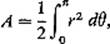
subject to the condition

4.6A uniform flexible cable of fixed length hangs between two fixed points. If it hangs in such a way as to minimize the height of its center of gravity, show that its shape is that of a catenary (see Example 2 of Section 3). Hint: Note that Exercise 3.2 applies.

4.7If a hanging flexible cable of fixed length supports a horizontally uniform load, show that its shape is that of a parabola.