5 Steps to a 5: AP Calculus AB 2017 (2016)

STEP 4

Review the Knowledge You Need to Score High

CHAPTER 12

Big Idea 3: Integrals and the Fundamental Theorems of Calculus

Definite Integrals

IN THIS CHAPTER

Summary: In this chapter, you will be introduced to the summation notation, the concept of a Riemann Sum, the Fundamental Theorems of Calculus, and the properties of definite integrals. You will also be shown techniques for evaluating definite integrals involving algebraic, trigonometric, logarithmic, and exponential functions. In addition, you will learn how to work with improper integrals. The ability to evaluate integrals is a prerequisite to doing well on the AP Calculus AB exam.

Key Ideas

Summation Notation

Riemann Sums

Properties of Definite Integrals

The First Fundamental Theorem of Calculus

The Second Fundamental Theorem of Calculus

Evaluating Definite Integrals

12.1 Riemann Sums and Definite Integrals

Main Concepts: Sigma Notation, Definition of a Riemann Sum, Definition of a Definite Integral, and Properties of Definite Integrals

Sigma Notation or Summation Notation

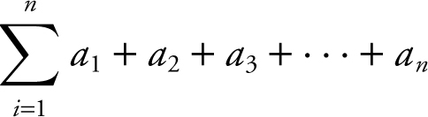
where i is the index of summation, l is the lower limit, and n is the upper limit of summation. (Note: The lower limit may be any non-negative integer ≤ n .)

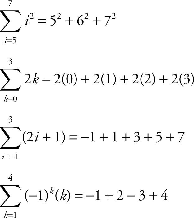
Examples

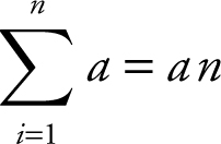
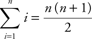
Summation Formulas

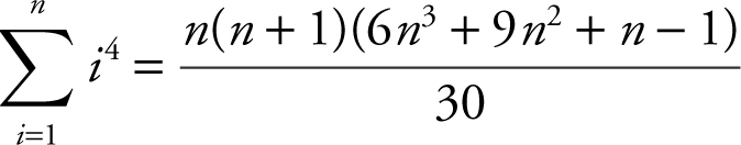
If n is a positive integer, then:

1.

2.

3.

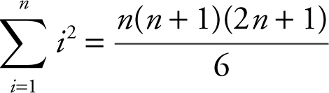
4.

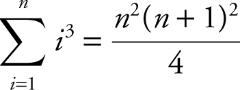
5.

Example

.

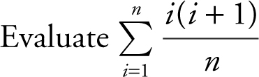(Note: This question has not appeared in an AP Calculus AB exam in recent years.)

• Remember: In exponential growth/decay problems, the formulas are 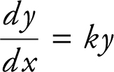and y = y ₀ e^kt .

Definition of a Riemann Sum

Let f be defined on [a , b ] and x_i be points on [a , b ] such that x ₀ = a , x_n = b , and a < x ₁ < x ₂ < x ₃ … < x _{n –1} < b . The points a , x ₁ , x ₂ , x ₃ , … x _{n –1} , and b form a partition of f denoted as Δ on [a , b ]. Let Δx_i be the length of the i th interval [x _{i –1} , x_i ] and c_i be any point in the i th interval. Then the Riemann sum of f for the partition is .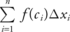

Example 1

Let f be a continuous function defined on [0, 12] as shown below.

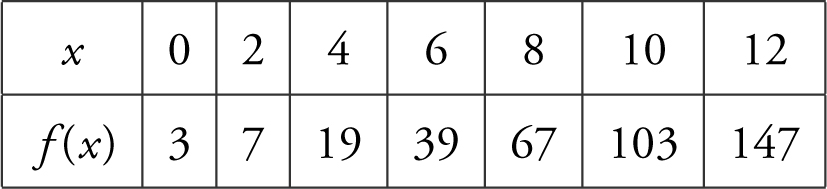
Find the Riemann sum for f (x ) over [0, 12] with 3 subdivisions of equal length and the midpoints of the intervals as c_i .

Length of an interval 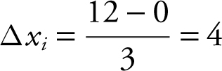. (See Figure 12.1-1 .)

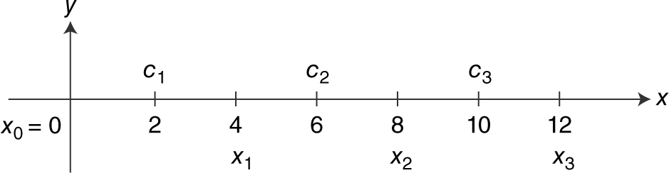
Figure 12.1-1

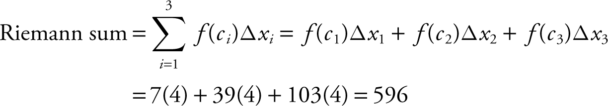
The Riemann sum is 596.

Example 2

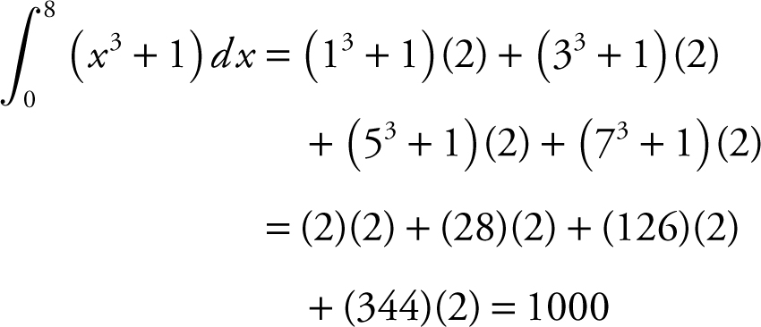
Find the Riemann sum for f (x ) = x ³ + 1 over the interval [0, 4] using 4 subdivisions of equal length and the midpoints of the intervals as c_i . (See Figure 12.1-2 .)

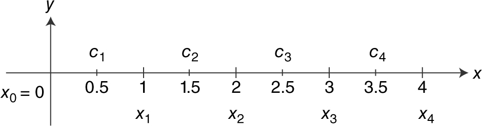
Figure 12.1-2

Length of an interval .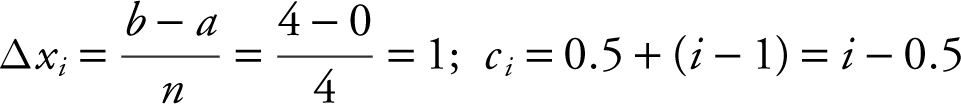

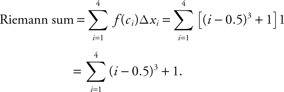
Enter Σ ((1 – 0.5)³ + 1, i , 1, 4) = 66.

The Riemann sum is 66.

Definition of a Definite Integral

Let f be defined on [a , b ] with the Riemann sum for f over [a , b ] written as .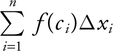

If max Δx_i is the length of the largest subinterval in the partition and the 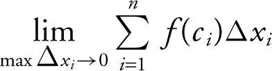exists, then the limit is denoted by:

.

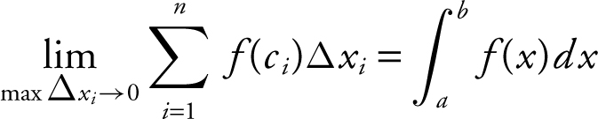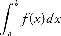is the definite integral of f from a to b .

Example 1

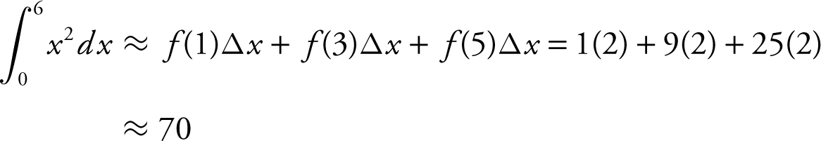
Use a midpoint Riemann sum with three subdivisions of equal length to find the approximate value of .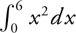

midpoints are x = 1, 3, and 5.

Example 2

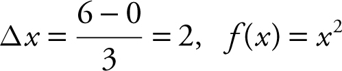
Using the limit of the Riemann sum, find .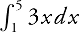

Using n subintervals of equal lengths, the length of an interval

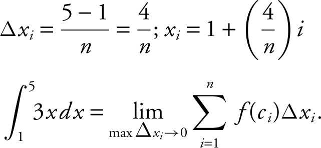
Let c_i = x_i ; max Δx_i → 0 ⇒ n → ∞.

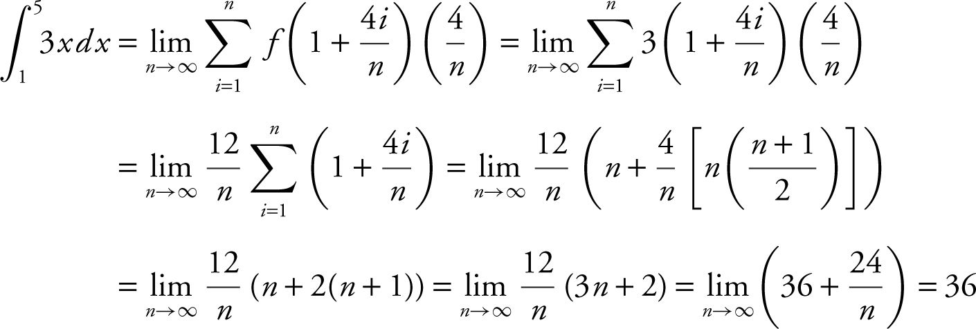
Thus,

(Note: This question has not appeared in an AP Calculus AB exam in recent years.)

Properties of Definite Integrals

1. If f is defined on [a , b ], and the exists, then f is integrable on [a , b ].

2. If f is continuous on [a , b ], then f is integrable on [a , b ].

If f (x ), g (x ), and h (x ) are integrable on [a , b ], then

3.

4.

5. when C is a constant.

6.

7. provided f (x ) ≥ 0 on [a , b ].

8. provided f (x ) ≥ g (x ) on [a , b ].

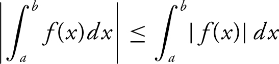
9.

10. 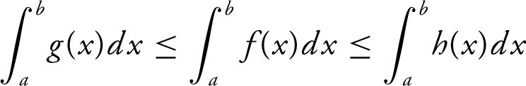; provided g (x ) ≤ f (x ) ≤ h (x ) on [a , b ].

11. 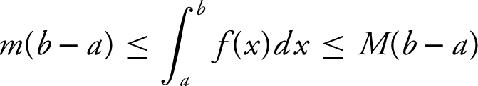; provided m ≤ f (x ) ≤ M on [a , b ].

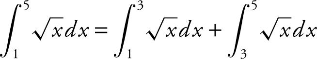
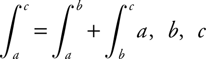
12. 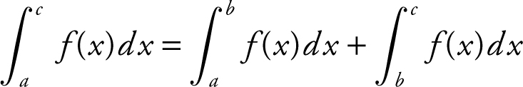; provided f (x ) is integrable on an interval containing a , b , c .

Examples

1.

2.

3.

4.

5.

Note: Or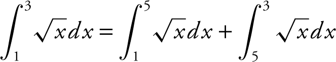

do not have to be arranged from smallest to largest.

The remaining properties are best illustrated in terms of the area under the curve of the function as discussed in the next section.

• Do not forget that .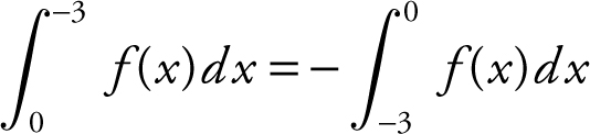

12.2 Fundamental Theorems of Calculus

Main Concepts: First Fundamental Theorem of Calculus, Second Fundamental Theorem of Calculus

First Fundamental Theorem of Calculus

If f is continuous on [a , b ] and F is an antiderivative of f on [a , b ], then

.

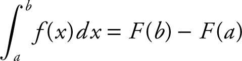Note: F (b ) – F (a ) is often denoted as .

Example 1

Evaluate .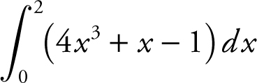

.

Example 2

Evaluate .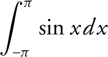

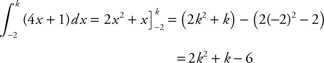
Example 3

If 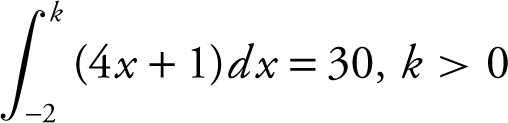, find k .

Example 4

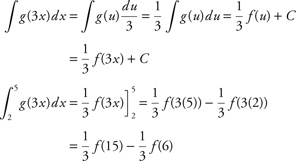
If f ′ (x ) = g (x ), and g is a continuous function for all real values of x , express 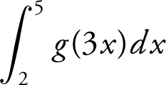in terms of f .

Let u = 3x ; du = 3dx or .

Example 5

Evaluate .

Cannot evaluate using the First Fundamental Theorem of Calculus since is discontinuous at x = 1.

Example 6

Using a graphing calculator, evaluate .

Using a TI-89 graphing calculator, enter and obtain 2π .

Second Fundamental Theorem of Calculus

If f is continuous on [a , b ] and 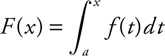, then F ′ (x ) = f (x ) at every point x in [a , b ].

Example 1

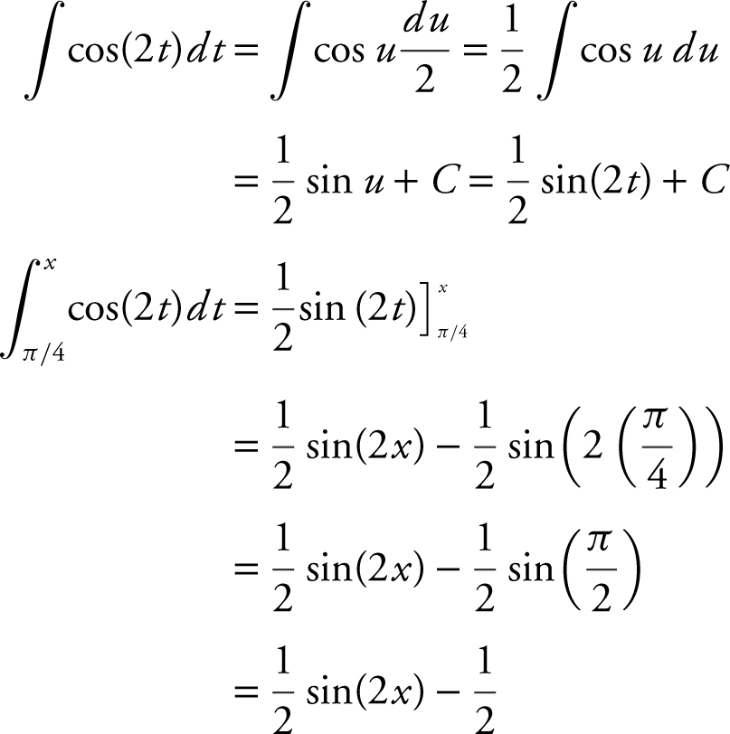
Evaluate .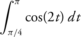

Let u = 2t ; du = 2dt or .

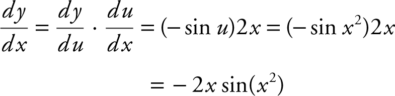
Example 2

Example 3

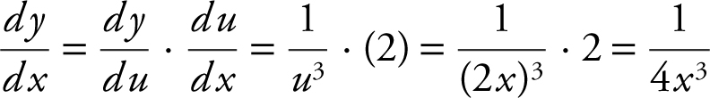
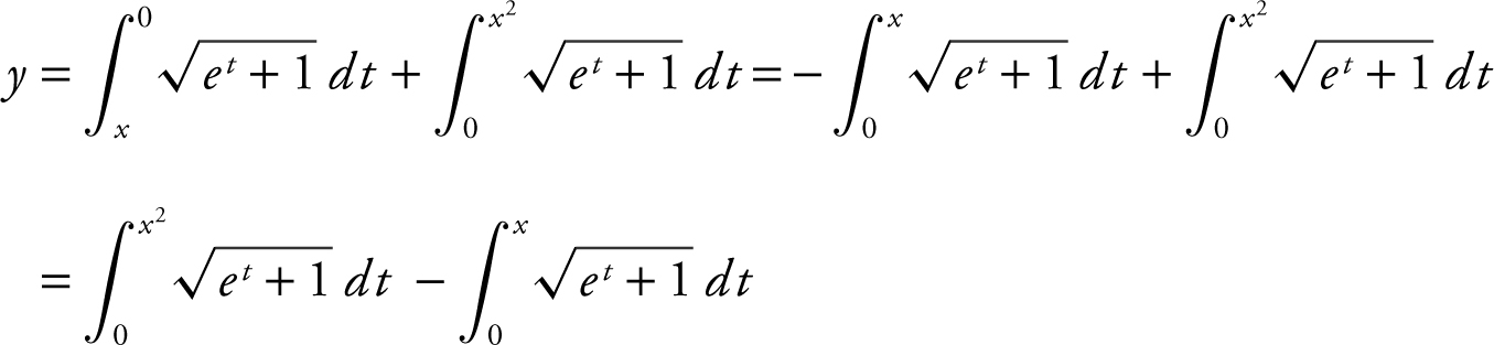
Find ; if y = .

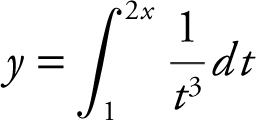Let u = 2x ; then .

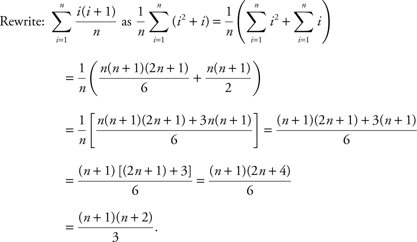
Rewrite: .

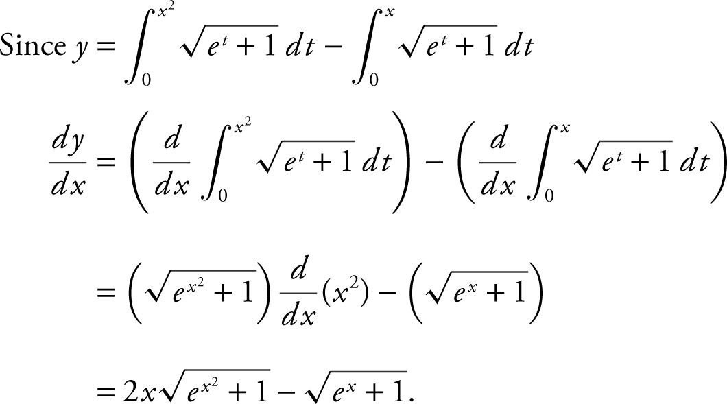
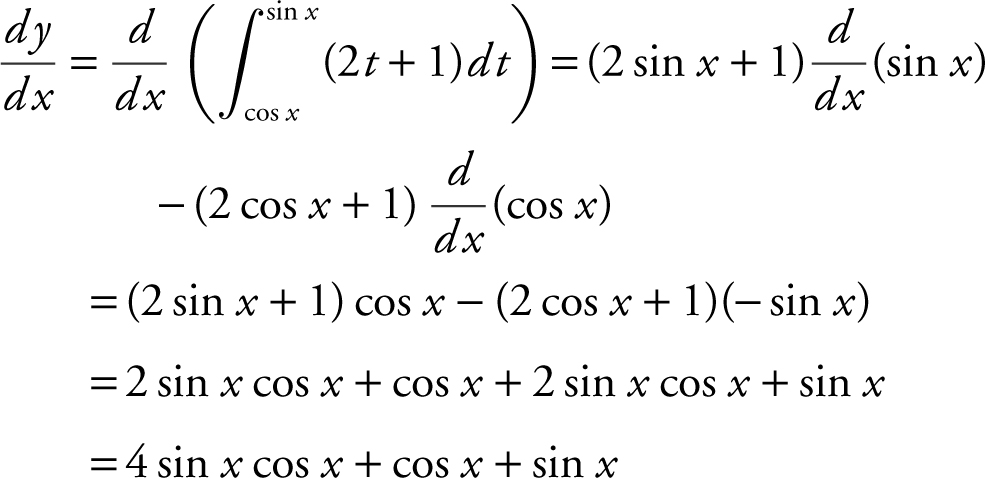
Example 4

Find ; if .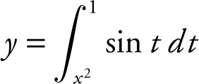

Rewrite: .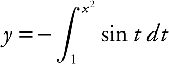

Let u = x ² ; then .

Rewrite: .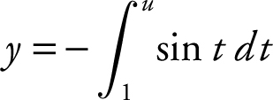

Example 5

Find 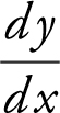; if .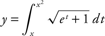

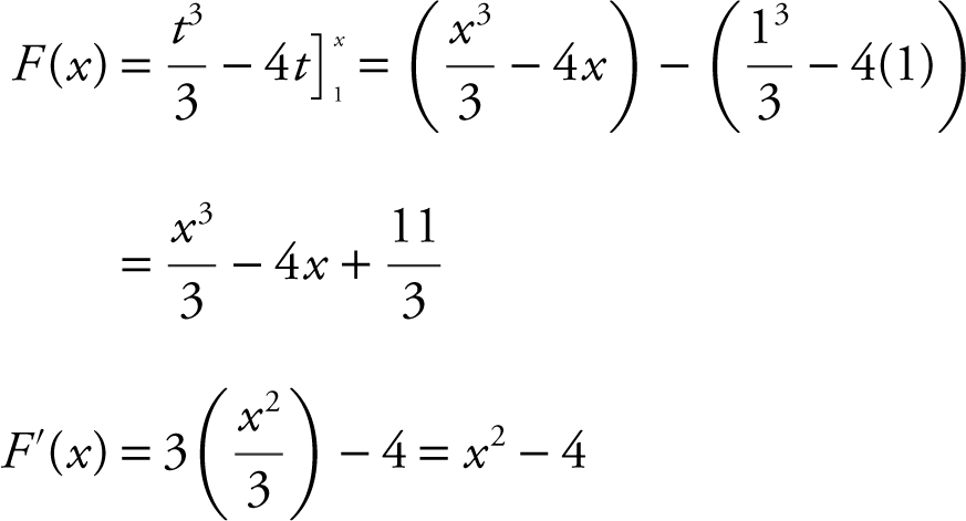
Example 6

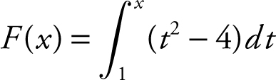, integrate to find F (x ) and then differentiate to find f ′ (x ).

12.3 Evaluating Definite Integrals

Main Concepts: Definite Integrals Involving Algebraic Functions; Definite Integrals Involving Absolute Value; Definite Integrals Involving Trigonometric, Logarithmic, and Exponential Functions; Definite Integrals Involving Odd and Even Functions

• If the problem asks you to determine the concavity of f ′ (not f ), you need to know if f ″ is increasing or decreasing, or if f ′″ is positive or negative.

Definite Integrals Involving Algebraic Functions

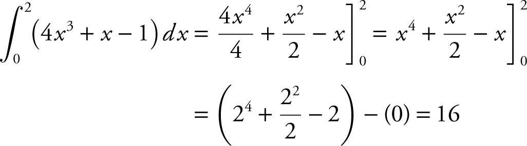
Example 1

Evaluate .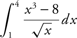

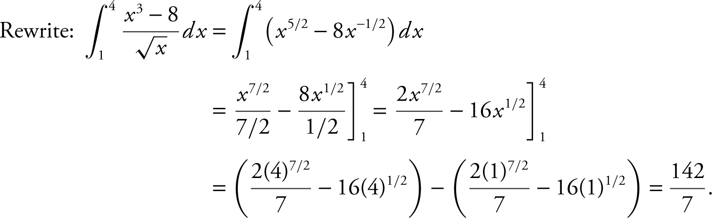
Verify your result with a calculator.

Example 2

Evaluate .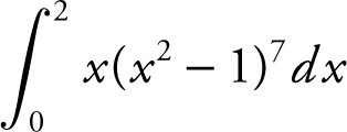

Begin by evaluating the indefinite integral .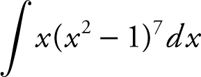

Let u = x ² – 1; du = 2x dx or .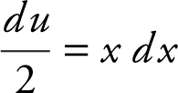

Rewrite: .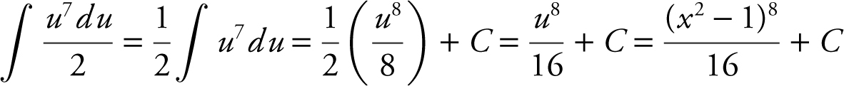

Thus the definite integral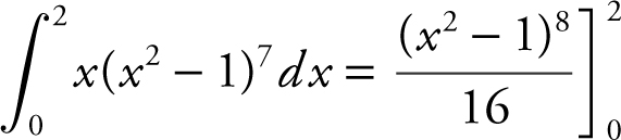

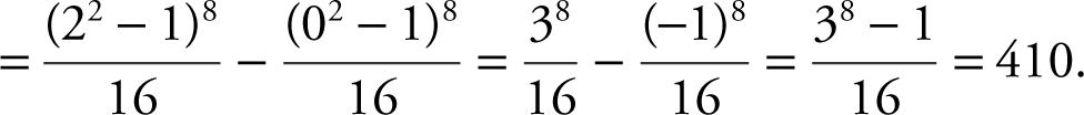
Verify your result with a calculator.

Example 3

Evaluate .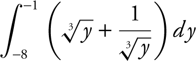

Rewrite: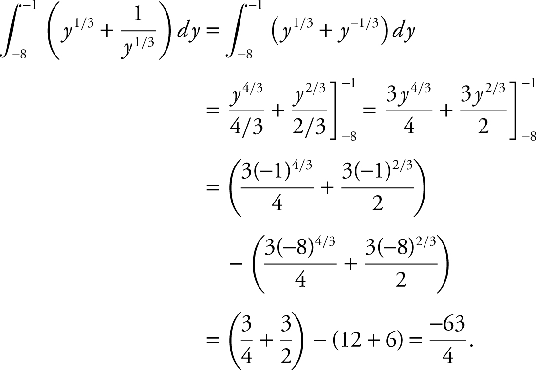

Verify your result with a calculator.

• You may bring up to 2 (but no more than 2) approved graphing calculators to the exam.

Definite Integrals Involving Absolute Value

Example 1

Evaluate .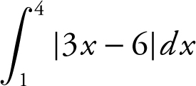

Set 3x – 6 = 0; x = 2; thus .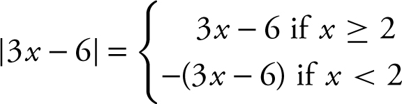

Rewrite integral:

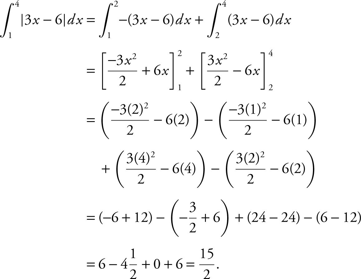
Verify your result with a calculator.

Example 2

Evaluate .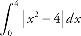

Set x ² – 4 = 0; x = ± 2.

Thus .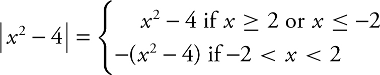

.

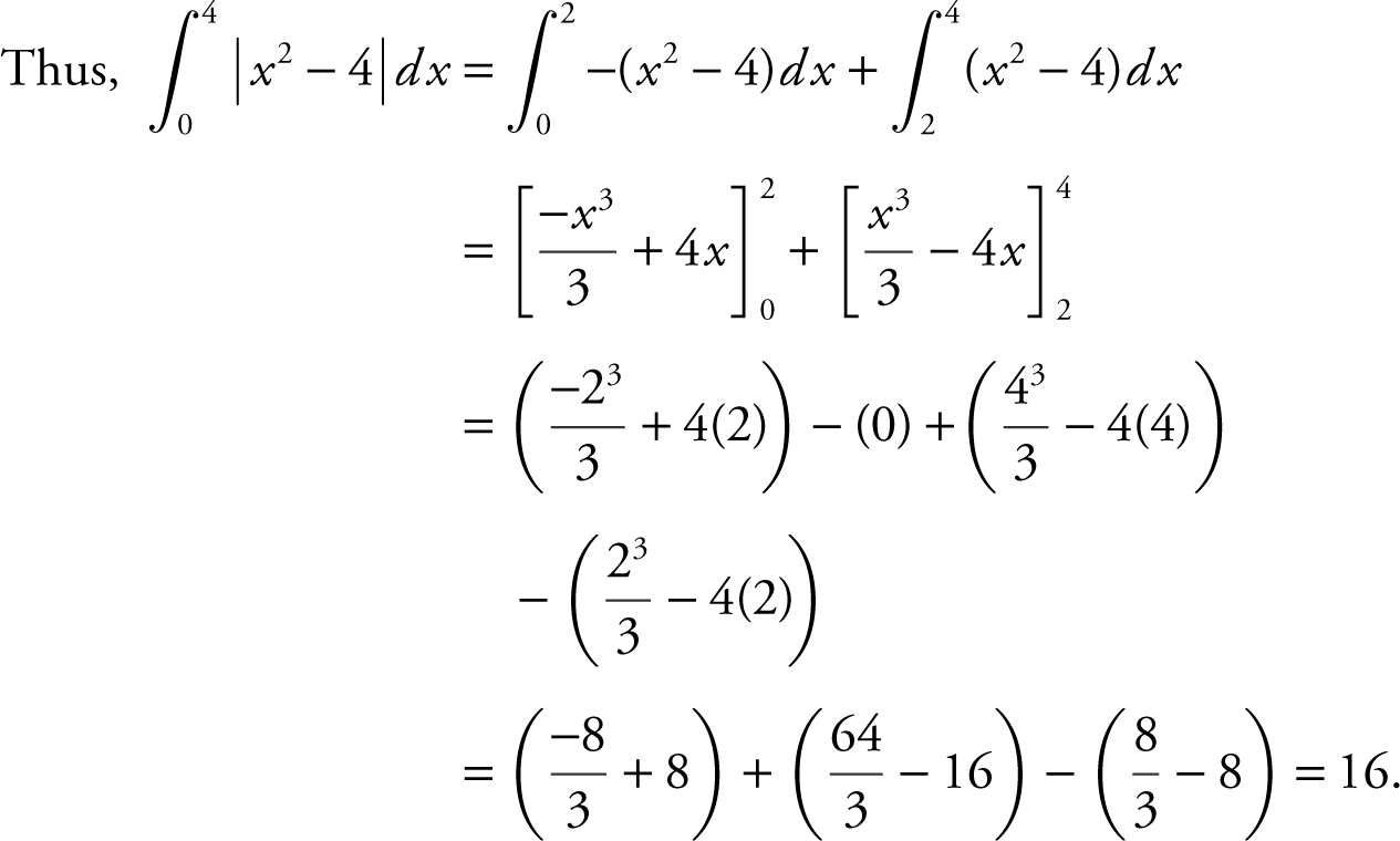Verify your result with a calculator.

• You are not required to clear the memories in your calculator for the exam.

Definite Integrals Involving Trigonometric, Logarithmic, and Exponential Functions

Example 1

Evaluate .

Rewrite: .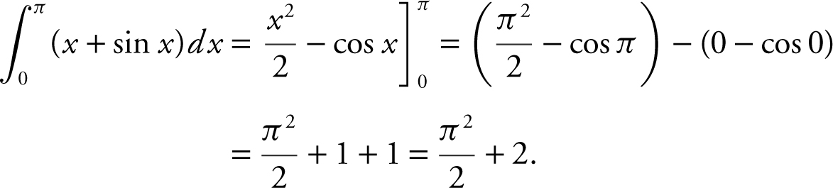

Verify your result with a calculator.

Example 2

Evaluate .

Let u = 3t ; du = 3dt or .

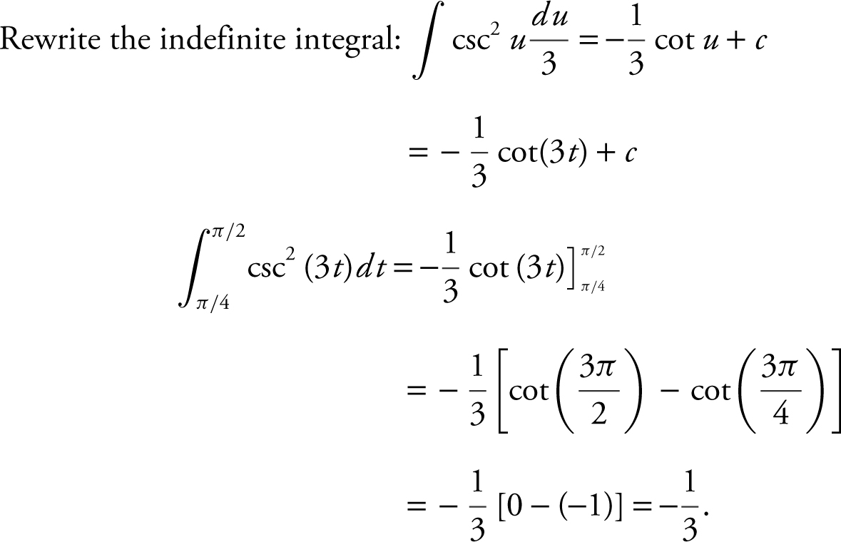
Verify your result with a calculator.

Example 3

.

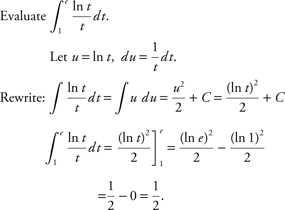Verify your result with a calculator.

Example 4

.

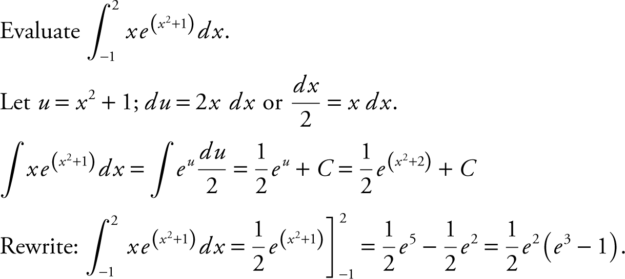Verify your result with a calculator.

Definite Integrals Involving Odd and Even Functions

If f is an even function, that is, f (–x ) = f (x ), and is continuous on [–a , a ], then

.

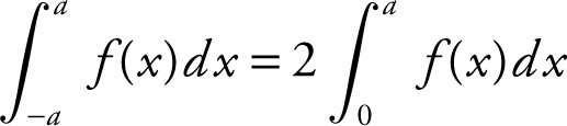If f is an odd function, that is, F (x ) = – f (–x ), and is continuous on [–a , a ], then

.

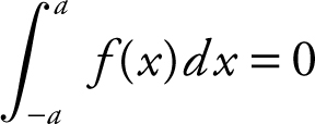Example 1

Evaluate .

Since f (x ) = cos x is an even function,

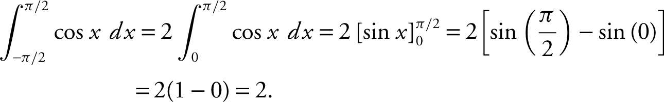
Verify your result with a calculator.

Example 2

Evaluate .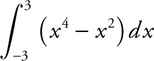

Since f (x ) = x ⁴ – x ² is an even function, i.e., f (–x ) = f (x ), thus

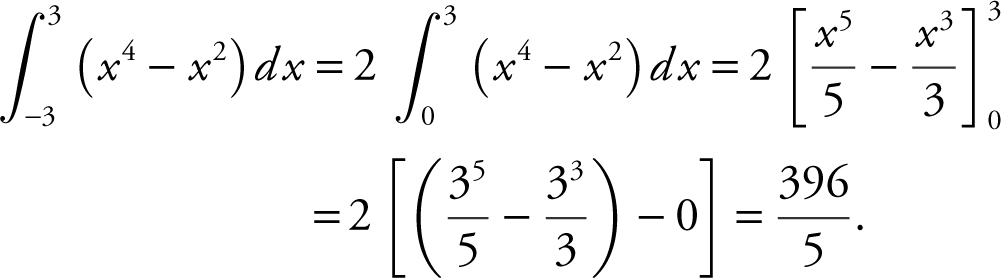
Verify your result with a calculator.

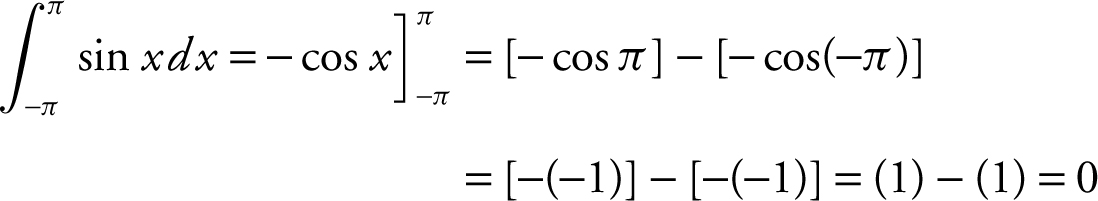
Example 3

Evaluate .

Since f (x ) = sin x is an odd function, i.e., f (–x ) = –f (x ), thus

.

Verify your result algebraically.

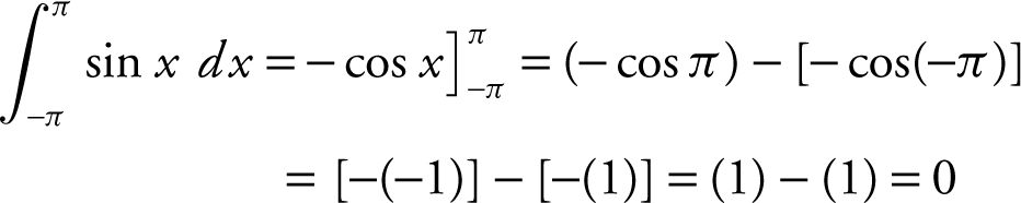
You can also verify the result with a calculator.

Example 4

If 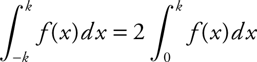for all values of k , then which of the following could be the graph of f ? (See Figure 12.3-1 .)

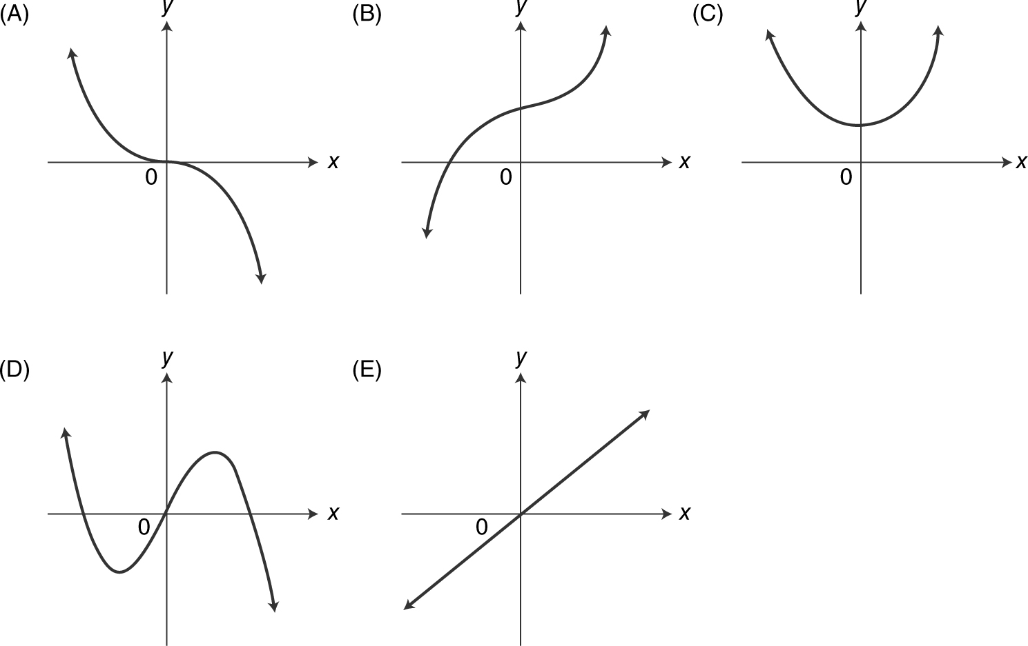
Figure 12.3-1

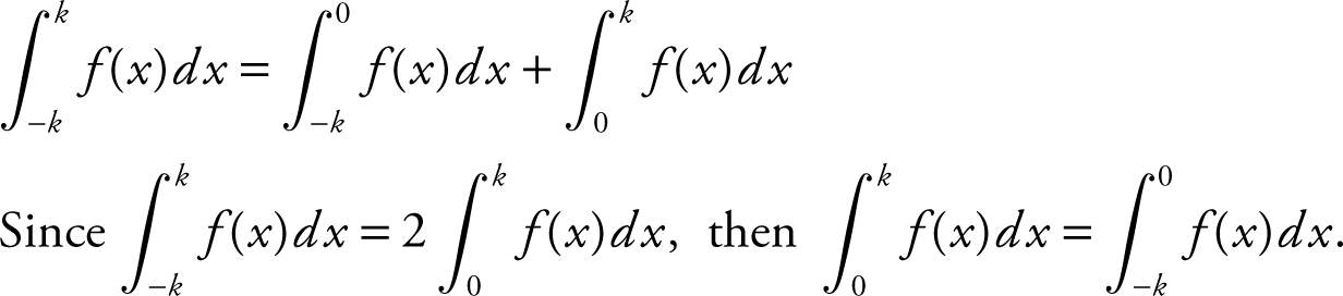
Thus f is an even function. Choice (C).

12.4 Rapid Review

1. Evaluate .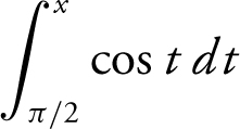

Answer: .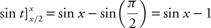

2. Evaluate .

Answer: .

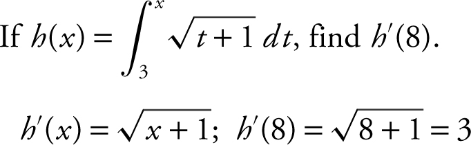
3. If , find G ′ (4).

Answer: G ′(x ) = (2x + 1)^3/2 and G ′ (4) = 9^3/2 = 27.

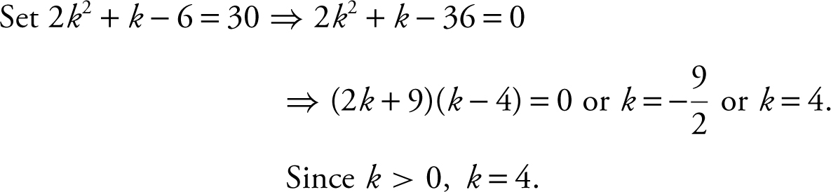
4. If , find k .

Answer: .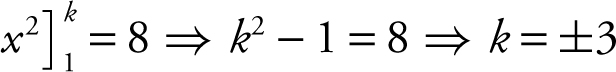

5. If G (x ) is an antiderivative of (e^x + 1) and G (0) = 0, find G (1).

Answer: G (x ) = e^x + x + C

G (0) = e ⁰ + 0 + C = 0 ⇒ C = –1.

G (1) = e ¹ + 1 – 1 = e .

6. If G ′ (x ) = g (x ), express 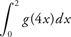in terms of G (x ).

Answer: Let .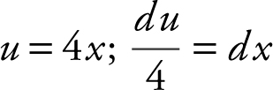

. Thus .

12.5 Practice Problems

Part A—The use of a calculator is not allowed .

Evaluate the following definite integrals.

1 .

2 .

3 .

4 .

5 . If = 4, find k .

6 .

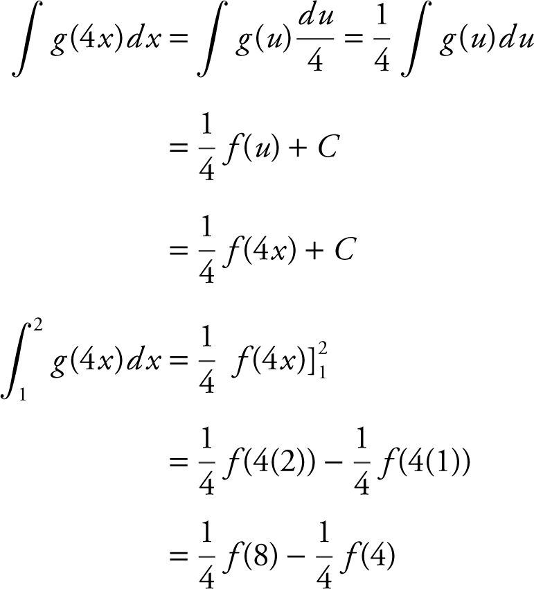
7 . If f ′ (x ) = g (x ) and g is a continuous function for all real values of x , express in terms of f .

8 .

9 .

10 . If 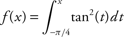(t )dt , find .

11 .

12 .

Part B—Calculators are allowed.

13 . Find k if .

14 . Evaluate to the nearest 100th.

15 . If , find .

16 . Use a midpoint Riemann sum with four subdivisions of equal length to find the approximate value of .

17 . Given

and , find

(a)

(b)

(c)

(d)

18 . Evaluate .

19 . Find if .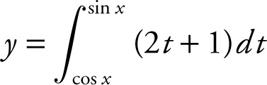

20 . Let f be a continuous function defined on [0, 30] with selected values as shown below:

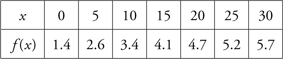
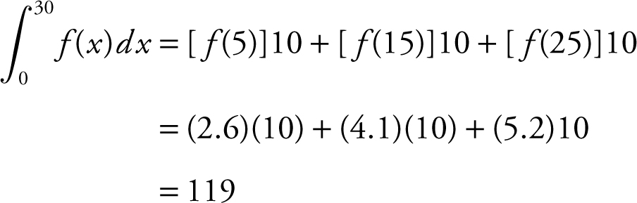
Use a midpoint Riemann sum with three subdivisions of equal length to find the approximate value of .

12.6 Cumulative Review Problems

(Calculator) indicates that calculators are permitted.

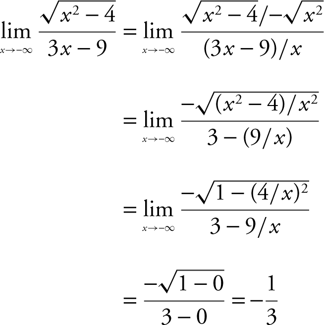
21 . Evaluate .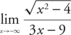

22 . Find at x = 3 if y = |x ² – 4|.

23 . The graph of f ′, the derivative of f , –6 ≤ x ≤ 8 is shown in Figure 12.6-1 .

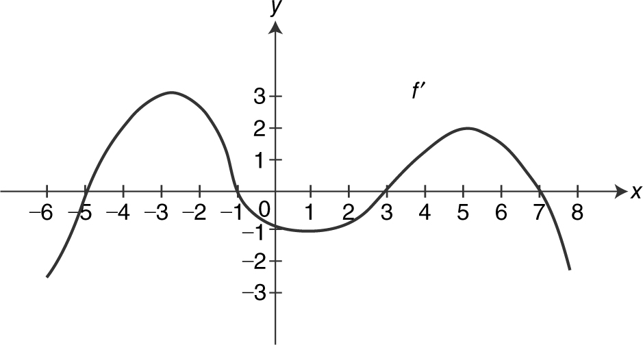
Figure 12.6-1

(a) Find all values of x such that f attains a relative maximum or a relative minimum.

(b) Find all values of x such that f is concave upward.

(c) Find all values of x such that f has a change of concavity.

24 . (Calculator) Given the equation 9x ² + 4y ² – 18x + 16y = 11, find the points on the graph where the equation has a vertical or horizontal tangent.

25 . (Calculator) Two corridors, one 6 feet wide and another 10 feet wide meet at a corner. (See Figure 12.6-2 .) What is the maximum length of a pipe of negligible thickness that can be carried horizontally around the corner?

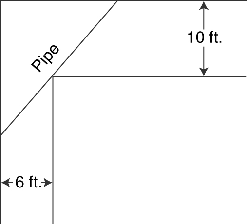
Figure 12.6-2

12.7 Solutions to Practice Problems

Part A—The use of a calculator is not allowed.

1 .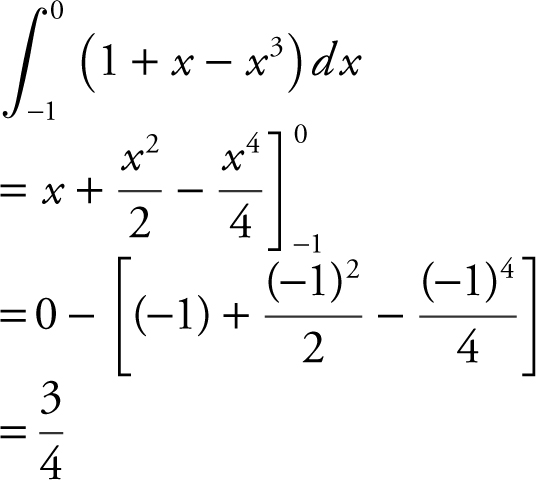

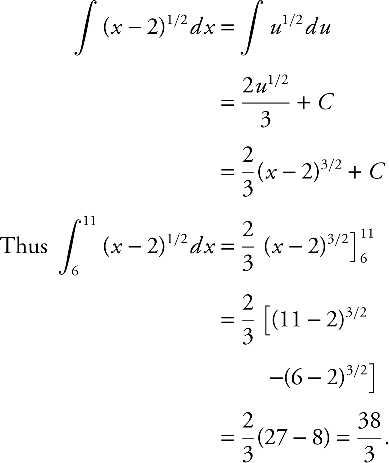
2 . Let u = x – 2 du = dx .

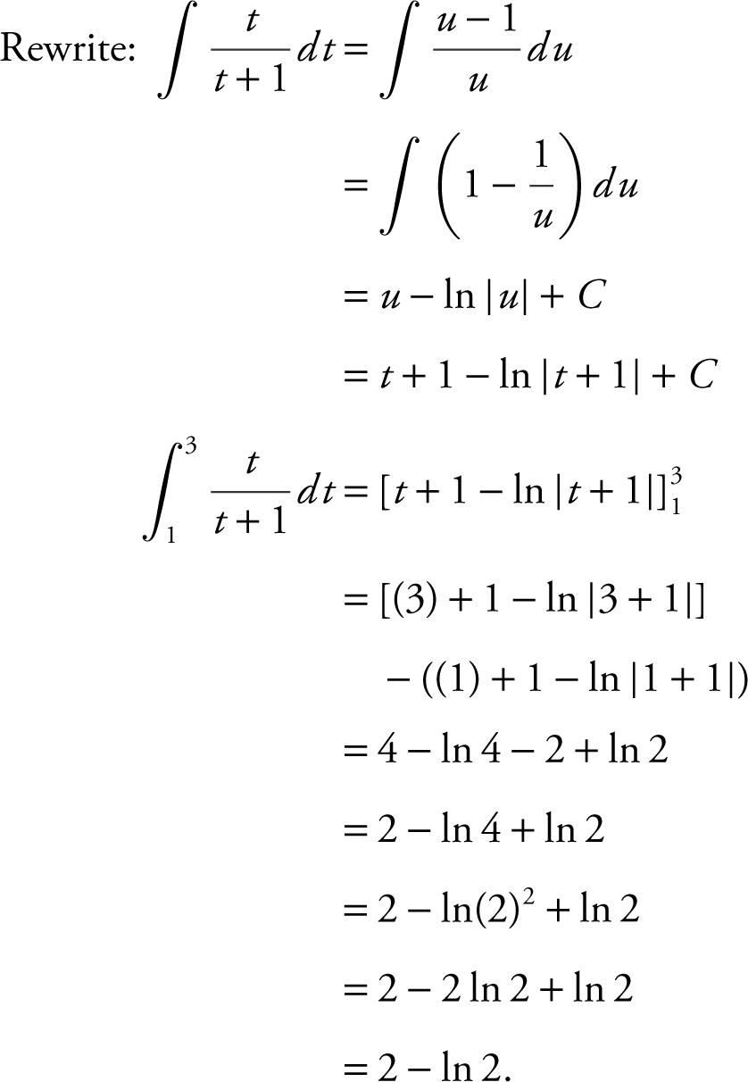
3 . Let u = t + 1; du = dt and t = u – 1.

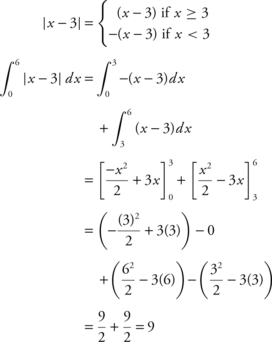
4 . Set x – 3 = 0; x = 3.

5 .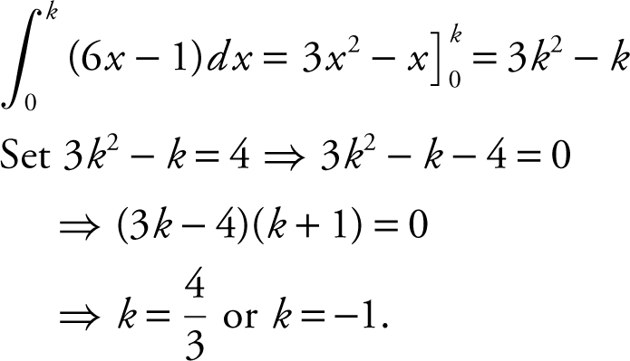

Verify your results by evaluating

.

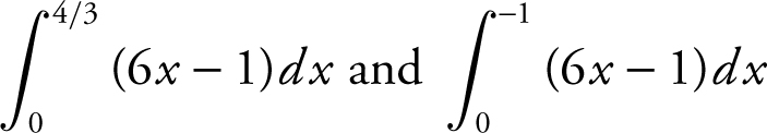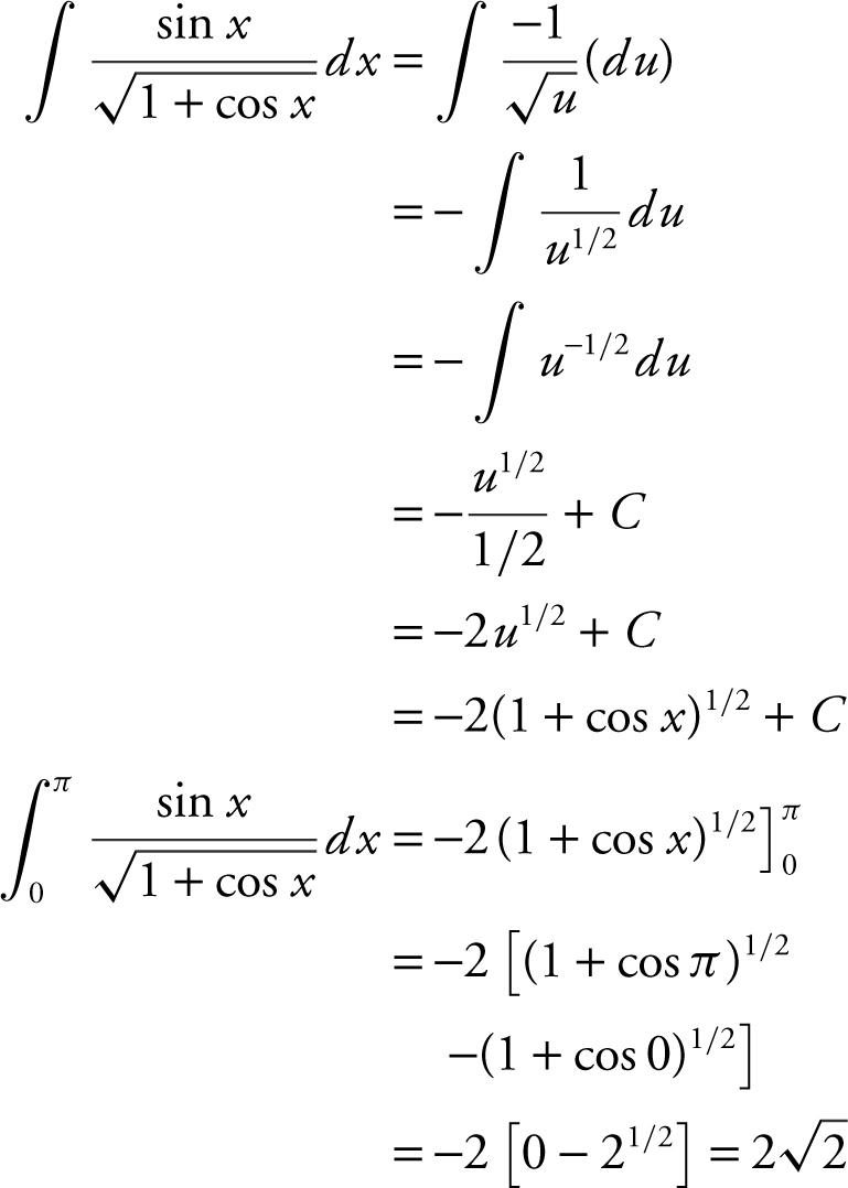
6 . Let u = 1 + cos x ; du = – sin x dx or – du = sin x dx .

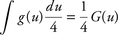
7 . Let u = 4x ; du = 4 dx or .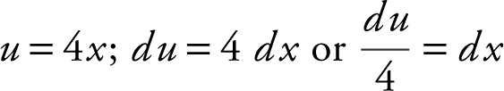

8 .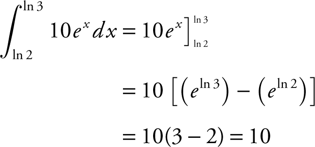

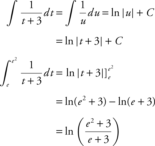
9 . Let u = t + 3; du = dt .

10 .

11 .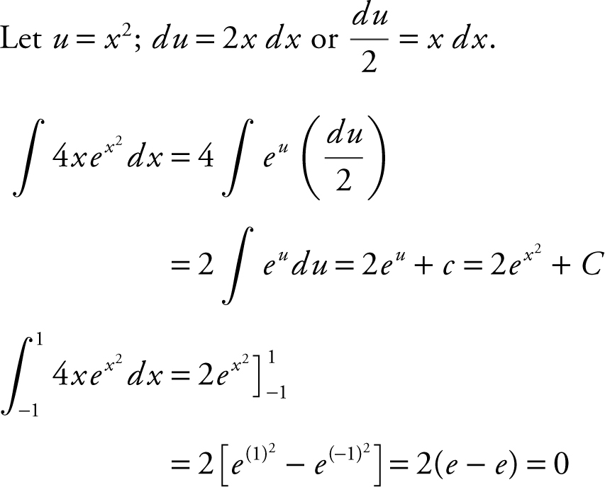

Note that f (x ) = 4xe ^{x 2} is an odd function.

Thus, .

12 .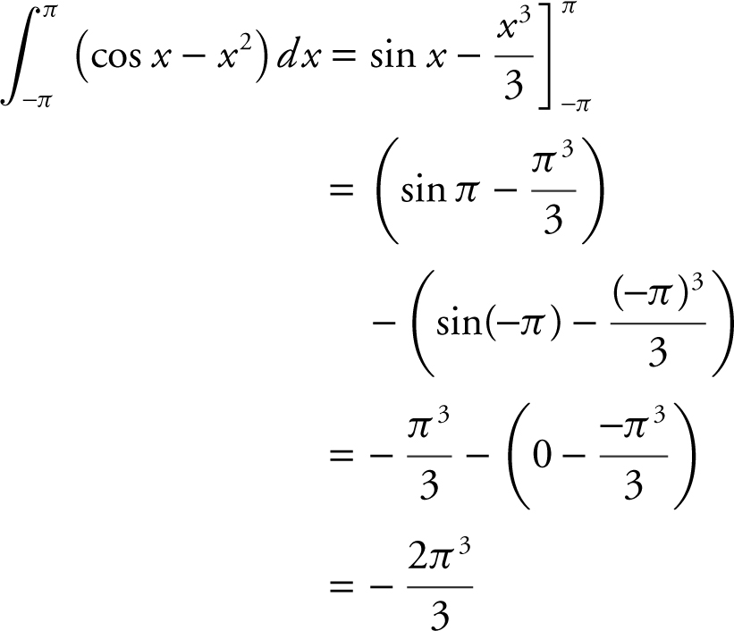

Note that f (x ) = cos x – x ² is an even function. Thus, you could have written 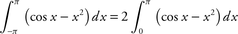and obtained the same result.

Part B—Calculators are allowed.

13 .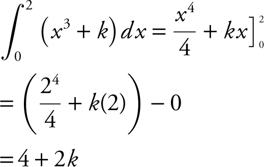

Set 4 + 2k = 10 and k = 3.

14 . Enter 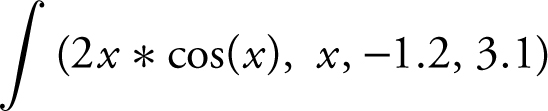and obtain – 4.70208 ≈ – 4.702.

15 .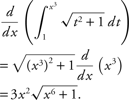

16 .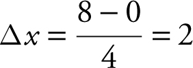

Midpoints are x = 1, 3, 5, and 7.

17 . (a)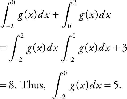

(b)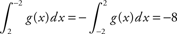

(c)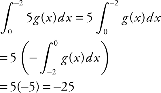

(d)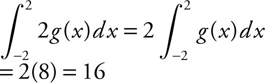

18 .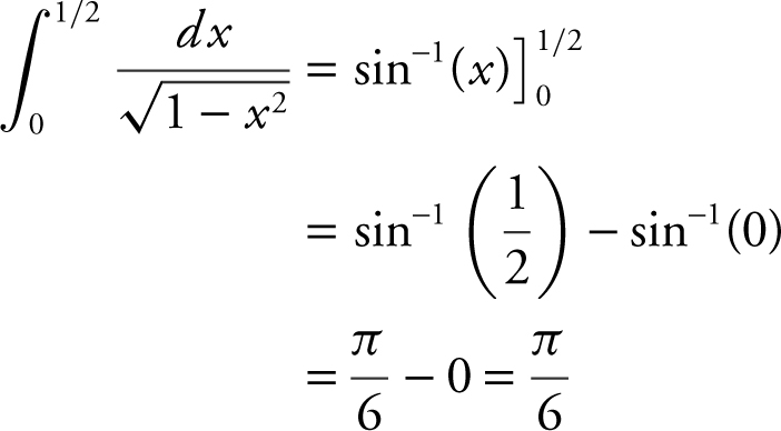

19 .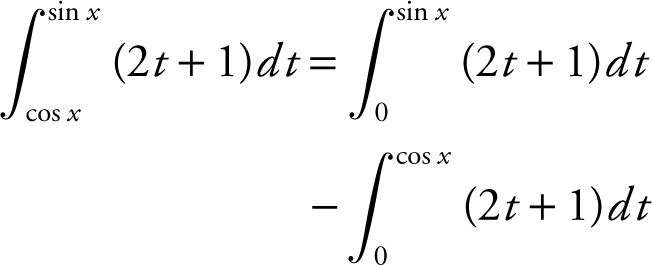

20 .

Midpoints are x = 5, 15, and 25.

12.8 Solutions to Cumulative Review Problems

21 . As x → –∞, .

22 .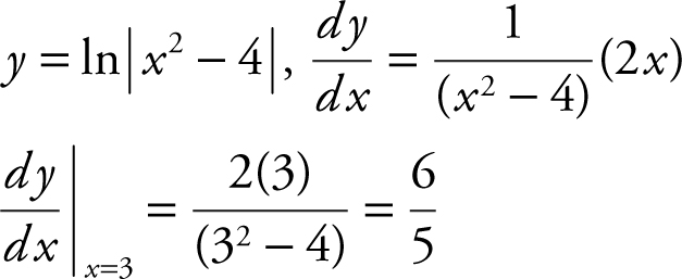

23 . (a) (See Figure 12.8-1 .)

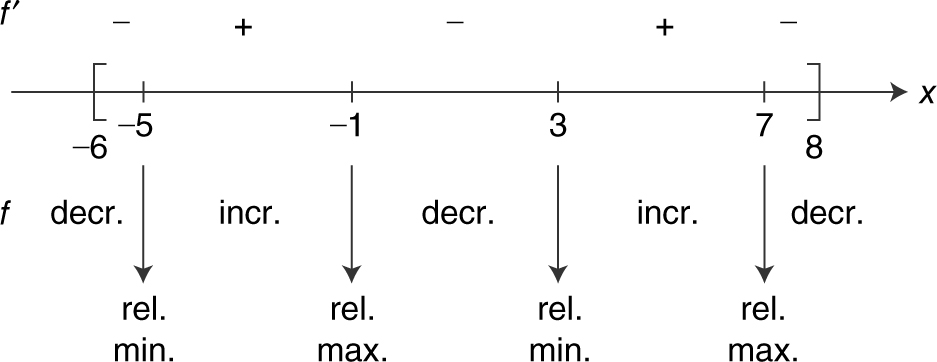
Figure 12.8-1

The function f has a relative minimum at x = – 5 and x = 3, and f has a relative maximum at x = – 1 and x = 7.

(b) (See Figure 12.8-2 .)

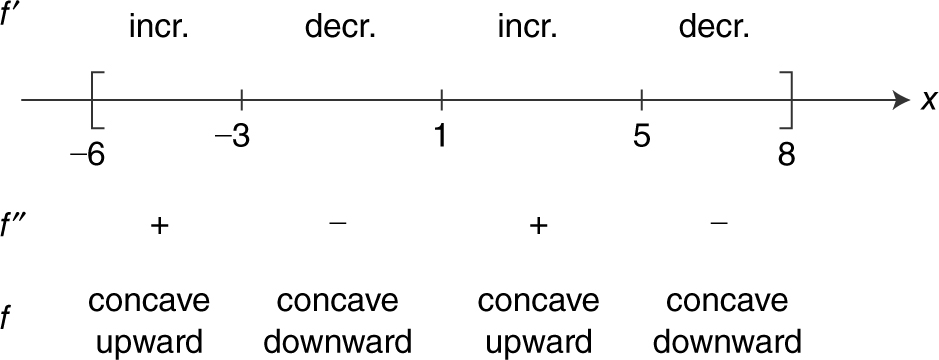
Figure 12.8-2

The function f is concave upward on intervals (– 6, – 3) and (1, 5).

(c) A change of concavity occurs at x = – 3, x = 1, and x = 5.

24 . (Calculator) Differentiate both sides of 9x ² + 4y ² – 18x + 16y = 11.

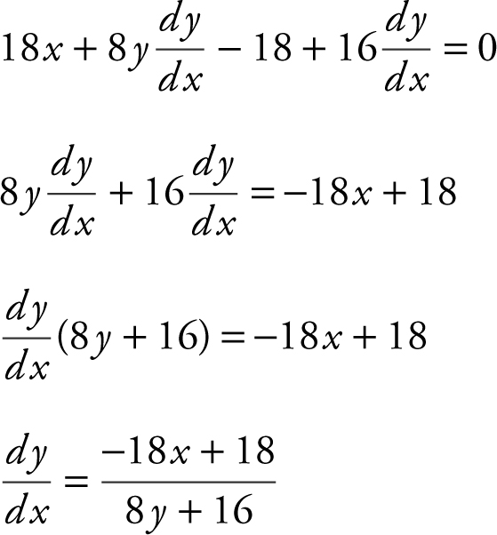
Horizontal tangent .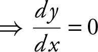

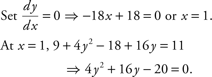
Using a calculator, enter [Solve ]

(4y ^∧ 2 + 16y – 20 = 0, y ); obtaining y = – 5 or y = 1.

Thus at each of the points at (1, 1) and (1, – 5) the graph has a horizontal tangent.

Vertical tangent is undefined.

Set 8y + 16 = 0 ⇒ y = – 2.

At y = – 2, 9x ² + 16 – 18x – 32 = 11

⇒ 9x ² – 18x – 27 = 0.

Enter [Solve ] (9x ² – 18x – 27 = 0, x ) and obtain x = 3or x = – 1.

Thus, at each of the points (3, – 2) and (– 1, – 2), the graph has a vertical tangent. (See Figure 12.8-3 .)

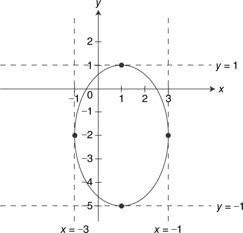
Figure 12.8-3

25 . (Calculator)

Step 1: (See Figure 12.8-4 .) Let P = x + y where P is the length of the pipe and x and y are as shown. The minimum value of P is the maximum length of the pipe to be able to turn in the corner. By similar triangles, 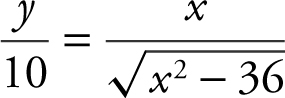and thus,

.

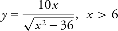
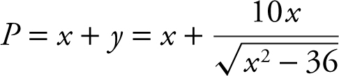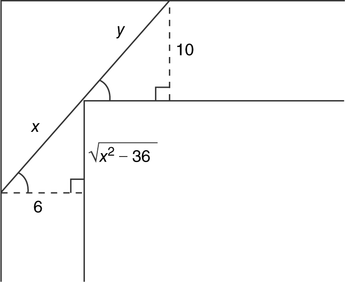
Figure 12.8-4

Step 2: Find the minimum value of P .

Enter 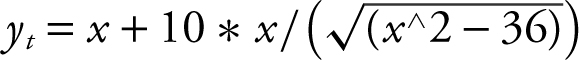. Use the [Minimum ] function of the calculator and obtain the minimum point (9.306, 22.388).

Step 3: Verify with the First Derivative Test.

Enter y 2 = (y 1(x ), x ) and observe. (See Figure 12.8-5 .)

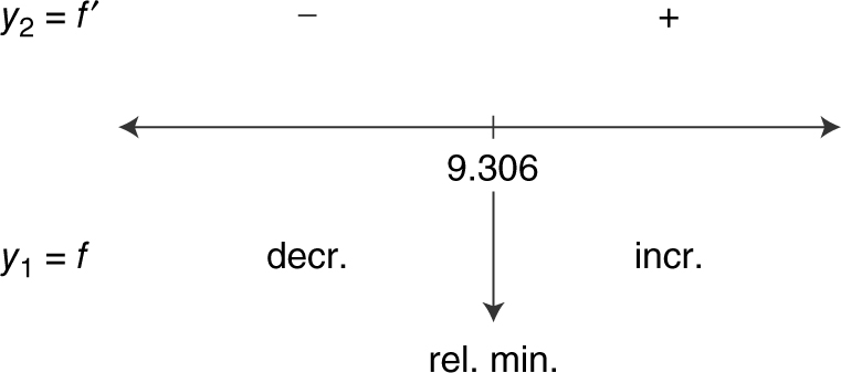
Figure 12.8-5

Step 4: Check endpoints.

The domain of x is (6, ∞). Since x = 9.306 is the only relative extremum, it is the absolute minimum. Thus the maximum length of the pipe is 22.388 feet.