Calculus For Dummies, 2nd Edition (2014)
Part II. Warming Up with Calculus Prerequisites
Chapter 5. Funky Functions and Their Groovy Graphs
IN THIS CHAPTER
Figuring out functions and relations
Learning about lines
Getting particular about parabolas
Grappling with graphs
Transforming functions and investigating inverse functions
Virtually everything you do in calculus concerns functions and their graphs in one way or another. Differential calculus involves finding the slope or steepness of various functions, and integral calculus involves computing the area underneath functions. And not only is the concept of a function critical for calculus, it’s one of the most fundamental ideas in all of mathematics.
What Is a Function?
Basically, a function is a relationship between two things in which the numerical value of one thing in some way depends on the value of the other. Examples are all around us: The average daily temperature for your city depends on, and is a function of, the time of year; the distance an object has fallen is a function of how much time has elapsed since you dropped it; the area of a circle is a function of its radius; and the pressure of an enclosed gas is a function of its temperature.
The defining characteristic of a function
 A function has only one output for each input.
Consider Figure 5-1.
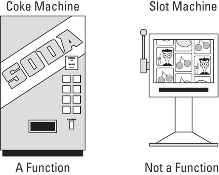
FIGURE 5-1: The Coke machine is a function. The slot machine is not.
The Coke machine is a function because after plugging in the inputs (your choice and your money), you know exactly what the output is. With the slot machine, on the other hand, the output is a mystery, so it’s not a function. Look at Figure 5-2.
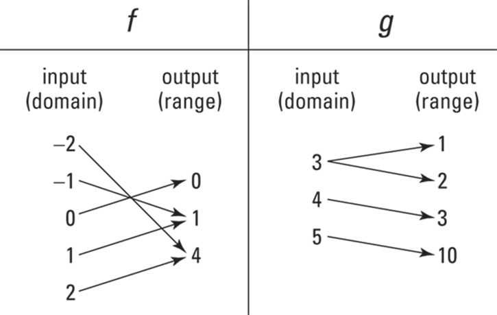
FIGURE 5-2: f is a function; g is not.
The squaring function, f, is a function because it has exactly one output assigned to each input. It doesn’t matter that both 2 and ![]() produce the same output of 4 because given an input, say
produce the same output of 4 because given an input, say ![]() , there’s no mystery about the output. When you input 3 into g, however, you don’t know whether the output is 1 or 2. (For now, don’t worry about how the g rule turns its inputs into its outputs.) Because no output mysteries are allowed in functions, g is not a function.
, there’s no mystery about the output. When you input 3 into g, however, you don’t know whether the output is 1 or 2. (For now, don’t worry about how the g rule turns its inputs into its outputs.) Because no output mysteries are allowed in functions, g is not a function.
Good functions, unlike good literature, have predictable endings.
Definitions of domain and range: The set of all inputs of a function is called the domain of the function; the set of all outputs is the range of the function.
Some people like to think of a function as a machine. Consider again the squaring function, f, from Figure 5-2. Figure 5-3 shows two of the inputs and their respective outputs.
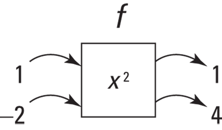
FIGURE 5-3: A function machine: Meat goes in, sausage comes out.
You pop a 1 into the function machine, and out pops a 1; you put in a ![]() and a 4 comes out. A function machine takes an input, operates on it in some way, then spits out the output.
and a 4 comes out. A function machine takes an input, operates on it in some way, then spits out the output.
Independent and dependent variables
Definitions of dependent variable and independent variable: In a function, the thing that depends on the other thing is called the dependent variable; the other thing is the independent variable. Because you plug numbers into the independent variable, it’s also called the input variable. After plugging in a number, you then calculate the output or answer for the dependent variable, so the dependent variable is also called the output variable. When you graph a function, the independent variable goes on the x-axis, and the dependent variable goes on the y-axis.
Sometimes the dependence between the two things is one of cause and effect — for example, raising the temperature of a gas causes an increase in the pressure. In this case, temperature is the independent variable and pressure the dependent variable because the pressure depends on the temperature.
Often, however, the dependence is not one of cause and effect, but just some sort of association between the two things. Usually, though, the independent variable is the thing we already know or can easily ascertain, and the dependent variable is the thing we want to figure out. For instance, you wouldn’t say that time causes an object to fall (gravity is the cause), but if you know how much time has passed since you dropped an object, you can figure out how far it has fallen. So, time is the independent variable, and distance fallen is the dependent variable; and you would say that distance is a function of time.
Whatever the type of correspondence between the two variables, the dependent variable (the y-variable) is the thing we’re usually more interested in. Generally, we want to know what happens to the dependent or y-variable as the independent or x-variable goes to the right: Is the y-variable (the height of the graph) rising or falling and, if so, how steeply, or is the graph level, neither going up nor down?
Function notation
A common way of writing the function ![]() is to replace the “y” with “
is to replace the “y” with “![]() ” and write
” and write ![]() . It’s just a different notation for the same thing. These two equations are, in every respect, mathematically identical. Students are often puzzled by function notation when they see it the first time. They wonder what the “f” is and whether
. It’s just a different notation for the same thing. These two equations are, in every respect, mathematically identical. Students are often puzzled by function notation when they see it the first time. They wonder what the “f” is and whether ![]() means f times x. It does not. If function notation bugs you, my advice is to think of
means f times x. It does not. If function notation bugs you, my advice is to think of ![]() as simply the way y is written in some foreign language. Don’t consider the f and the x separately; just think of
as simply the way y is written in some foreign language. Don’t consider the f and the x separately; just think of ![]() as a single symbol for y.
as a single symbol for y.
You can also think of ![]() (read as “f of x”) as short for “a function of x.” You can write
(read as “f of x”) as short for “a function of x.” You can write ![]() , which is translated as “y is a function of x and that function is
, which is translated as “y is a function of x and that function is ![]() .” However, sometimes other letters are used instead of f — such as
.” However, sometimes other letters are used instead of f — such as ![]() or
or ![]() — often just to differentiate between functions. The function letter doesn’t necessarily stand for anything, but sometimes the initial letter of a word is used (in which case you use an uppercase letter). For instance, you know that the area of a square is determined by squaring the length of its side:
— often just to differentiate between functions. The function letter doesn’t necessarily stand for anything, but sometimes the initial letter of a word is used (in which case you use an uppercase letter). For instance, you know that the area of a square is determined by squaring the length of its side: ![]() or
or ![]() . The area of a square depends on, and is a function of, the length of its side. With function notation, you can write
. The area of a square depends on, and is a function of, the length of its side. With function notation, you can write ![]() . (Quick quiz: How does
. (Quick quiz: How does ![]() differ from the area of a square function,
differ from the area of a square function, ![]() ? Answer: For
? Answer: For ![]() , x can equal any number, but with
, x can equal any number, but with ![]() , s must be positive, because the length of a side of a square cannot be negative or zero. The two functions thus have different domains.)
, s must be positive, because the length of a side of a square cannot be negative or zero. The two functions thus have different domains.)
Consider, again, the squaring function ![]() or
or ![]() . When you input 3 for x, the output is 9. Function notation is convenient because you can concisely express the input and the output by writing
. When you input 3 for x, the output is 9. Function notation is convenient because you can concisely express the input and the output by writing ![]() (read as “f of 3 equals 9”). Remember that
(read as “f of 3 equals 9”). Remember that ![]() means that when x is 3,
means that when x is 3, ![]() is 9; or, equivalently, it tells you that when x is 3, y is 9.
is 9; or, equivalently, it tells you that when x is 3, y is 9.
Composite functions
A composite function is the combination of two functions. For example, the cost of the electrical energy needed to air condition your place depends on how much electricity you use, and usage depends on the outdoor temperature. Because cost depends on usage and usage depends on temperature, cost will depend on temperature. In function language, cost is a function of usage, usage is a function of temperature, and thus cost is a function of temperature. This last function, a combination of the first two, is a composite function.
Let ![]() and
and ![]() . Input 3 into
. Input 3 into ![]() , which equals 7. Now take that output, 7, and plug it into
, which equals 7. Now take that output, 7, and plug it into ![]() . The machine metaphor shows what I did here. Look at Figure 5-4. The gmachine turns the 3 into a 7, and then the f machine turns the 7 into a 49.
. The machine metaphor shows what I did here. Look at Figure 5-4. The gmachine turns the 3 into a 7, and then the f machine turns the 7 into a 49.
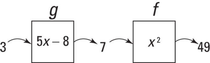
FIGURE 5-4: Two function machines.
You can express the net result of the two functions in one step with the following composite function:
![]()
You always calculate the inside function of a composite function first: ![]() . Then you take the output, 7, and calculate
. Then you take the output, 7, and calculate ![]() , which equals 49.
, which equals 49.
To determine the general composite function, ![]() , plug
, plug ![]() , which equals
, which equals ![]() , into
, into ![]() . In other words, you want to determine
. In other words, you want to determine ![]() . The f function or f machine takes an input and squares it. Thus,
. The f function or f machine takes an input and squares it. Thus,
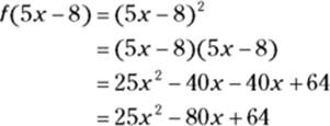
Thus, ![]() .
.
 With composite functions, the order matters. As a general rule,
 ![]() .
.
What Does a Function Look Like?
I’m no math historian, but everyone seems to agree that René Descartes (1596–1650) came up with the x-y coordinate system shown in Figure 5-5.
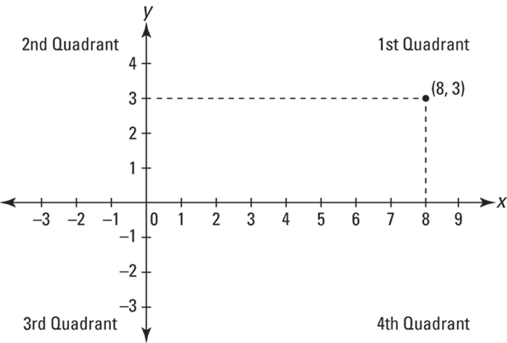
FIGURE 5-5: The Cartesian (for Descartes) or x-y coordinate system.
Isaac Newton (1642–1727) and Gottfried Leibniz (1646–1716) are credited with inventing calculus, but it’s hard to imagine that they could have done it without Descartes’ contribution several decades earlier. Think of the coordinate system (or the screen on your graphing calculator) as your window into the world of calculus. Virtually everything in your calculus textbook and in this book involves (directly or indirectly) the graphs of lines or curves — usually functions — in the x-y coordinate system.
Consider the four graphs in Figure 5-6.
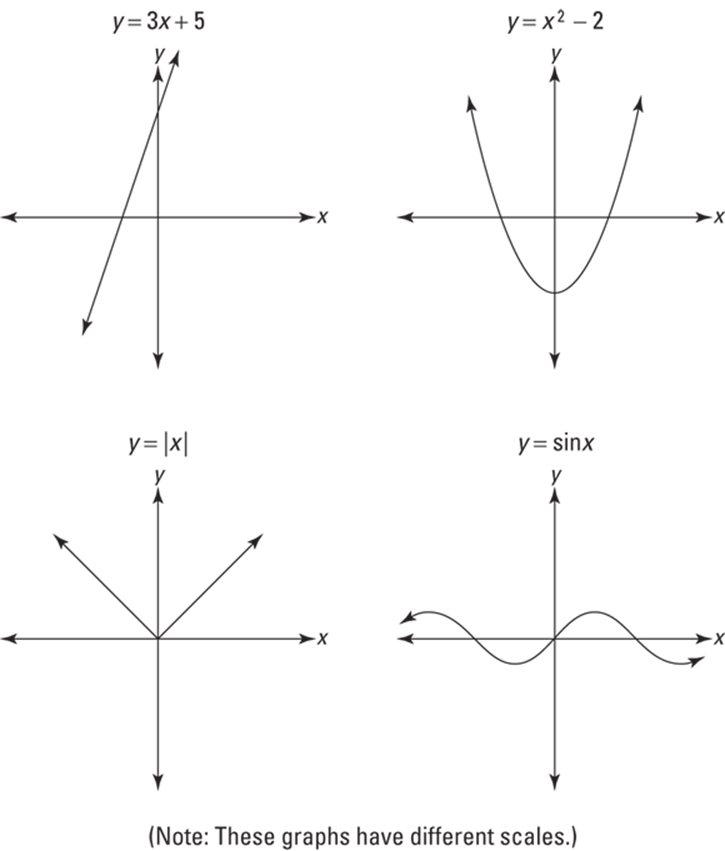
FIGURE 5-6: Four functions.
These four curves are functions because they satisfy the vertical line test. (Note: I’m using the term curve here to refer to any shape, whether it’s curved or straight.)
The vertical line test: A curve is a function if a vertical line drawn through the curve — regardless of where it’s drawn — touches the curve only once. This guarantees that each input within the function’s domain has exactly one output.
No matter where you draw a vertical line on any of the four graphs in Figure 5-6, the line touches the curve at only one point. Try it.
If, however, a vertical line can be drawn so that it touches a curve two or more times, then the curve is not a function. The two curves in Figure 5-7, for example, are not functions.
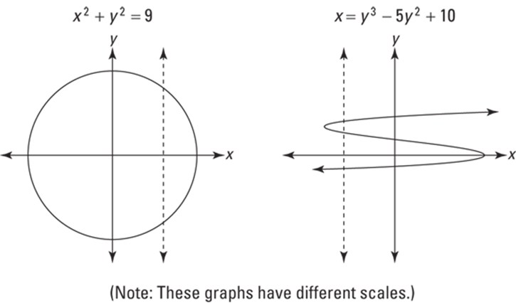
FIGURE 5-7: These two curves are not functions because they fail the vertical line test. They are, however, relations.
So, the four curves in Figure 5-6 are functions, and the two in Figure 5-7 are not, but all six of the curves are relations.
Definition of relation: A relation is any collection of points on the x-y coordinate system.
You spend a little time studying some non–function relations in calculus — circles, for instance — but the vast majority of calculus problems involve functions.
Common Functions and Their Graphs
You’re going to see hundreds of functions in your study of calculus, so it wouldn’t be a bad idea to familiarize yourself with the basic ones in this section: the line, the parabola, the absolute value function, the cubing and cube root functions, and the exponential and logarithmic functions.
Lines in the plane in plain English
A line is the simplest function you can graph on the coordinate plane. (Lines are important in calculus because you often study lines that are tangent to curves and because when you zoom in far enough on a curve, it looks and behaves like a line.) Figure 5-8 shows an example of a line: ![]() .
.
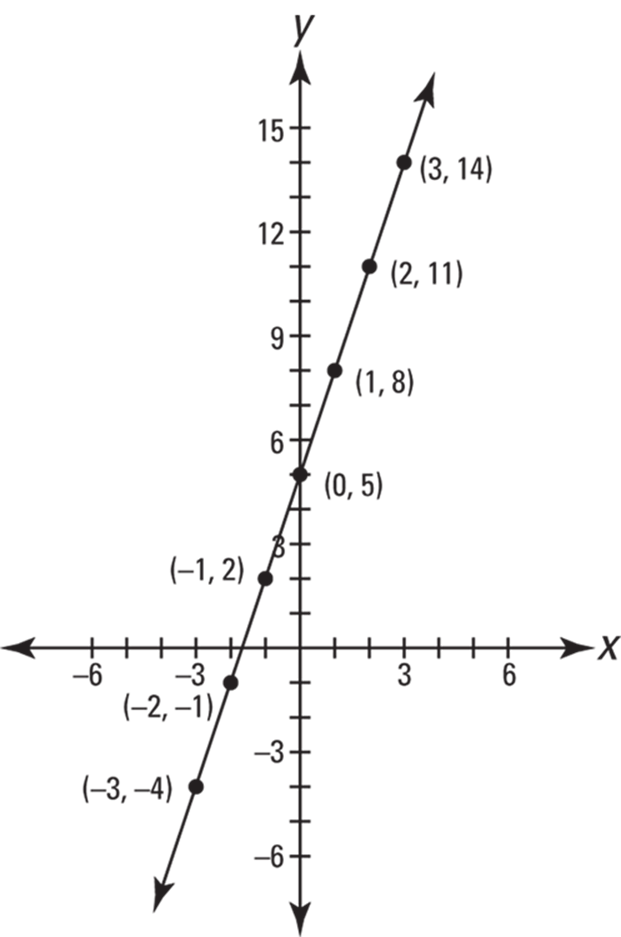
FIGURE 5-8: The graph of the line ![]()
Hitting the slopes
The most important thing about the line in Figure 5-8 — at least for your study of calculus — is its slope or steepness. Notice that whenever x goes 1 to the right, y goes up by 3. A good way to visualize slope is to draw a stairway under the line (see Figure 5-9). The vertical part of the step is called the rise, the horizontal part is called the run, and the slope is defined as the ratio of the rise to the run:
![]()
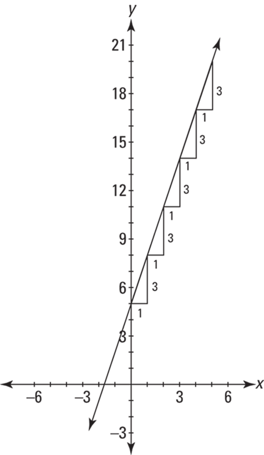
FIGURE 5-9: The line ![]() has a slope of 3.
has a slope of 3.
You don’t have to make the run equal to 1. The ratio of rise to run, and thus the slope, always comes out the same, regardless of what size you make the steps. If you make the run equal to 1, however, the slope is the same as the rise because a number divided by 1 equals itself. This is a good way to think about slope — the slope is the amount that a line goes up (or down) as it goes 1 to the right.
Definitions of positive, negative, zero, and undefined slopes: Lines that go up to the right have a positive slope; lines that go down to the right have a negative slope. Horizontal lines have a slope of zero, and vertical lines do not have a slope — you say that the slope of a vertical line is undefined.
Here’s the formula for slope:
![]()
Pick any two points on the line in Figure 5-9, say ![]() and
and ![]() , and plug them into the formula to calculate the slope:
, and plug them into the formula to calculate the slope:
![]()
This computation involves, in a sense, a stairway step that goes over 2 and up 6. The answer of 3 agrees with the slope you can see in Figure 5-9.
Any line parallel to this one has the same slope, and any line perpendicular to this one has a slope of ![]() , which is the opposite reciprocal of 3.
, which is the opposite reciprocal of 3.
Parallel lines have the same slope. Perpendicular lines have opposite reciprocal slopes.
Graphing lines
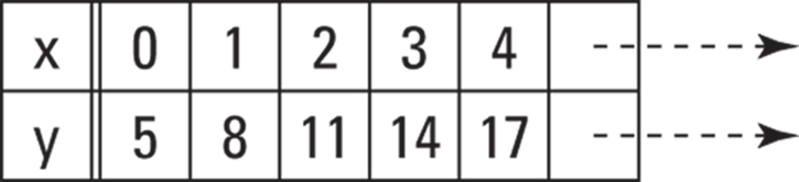
If you have the equation of the line, ![]() , but not its graph, you can graph the line the old-fashioned way or with your graphing calculator. The old-fashioned way is to create a table of values by plugging numbers into xand calculating y. If you plug 0 into x, y equals 5; plug 1 into x, and y equals 8; plug 2 into x, and y is 11, and so on. Table 5-1 shows the results.
, but not its graph, you can graph the line the old-fashioned way or with your graphing calculator. The old-fashioned way is to create a table of values by plugging numbers into xand calculating y. If you plug 0 into x, y equals 5; plug 1 into x, and y equals 8; plug 2 into x, and y is 11, and so on. Table 5-1 shows the results.
TABLE 5-1 Points on the Line y = 3x + 5
Plot the points, connect the dots, and put arrows on both ends — there’s your line. This is a snap with a graphing calculator. Just enter ![]() and your calculator graphs the line and produces a table like Table 5-1.
and your calculator graphs the line and produces a table like Table 5-1.
Slope-intercept and point-slope forms
You can see that the line in Figure 5-9 crosses the y-axis at 5 — this point is the y-intercept of the line. Because both the slope of 3 and the y-intercept of 5 appear in the equation ![]() , this equation is said to be in slope-intercept form. Here’s the form written in the general way:
, this equation is said to be in slope-intercept form. Here’s the form written in the general way:
Slope-intercept form:
![]()
(Where m is the slope and b is the y-intercept.)
(If that doesn’t ring a bell — even a distant, faint bell — go directly to the registrar and drop calculus, but do not under any circumstances return this book.)
All lines, except for vertical lines, can be written in this form. Vertical lines are written like ![]() , for example. The number tells you where the vertical line crosses the x–axis.
, for example. The number tells you where the vertical line crosses the x–axis.
The equation of a horizontal line also looks different, ![]() for example. But it technically fits the form
for example. But it technically fits the form ![]() — it’s just that because the slope of a horizontal line is zero, and because zero times x is zero, there is no x-term in the equation. (But, if you felt like it, you could write
— it’s just that because the slope of a horizontal line is zero, and because zero times x is zero, there is no x-term in the equation. (But, if you felt like it, you could write ![]() as
as ![]() .)
.)
 Definition of a constant function: A line is the simplest type of function, and a horizontal line (called a constant function) is the simplest type of line. It’s nonetheless fairly important in calculus, so make sure you know that a horizontal line has an equation like
 ![]() and that its slope is zero.
and that its slope is zero.
If ![]() and
and ![]() , you get the function
, you get the function ![]() . This line goes through the origin
. This line goes through the origin ![]() and makes a 45° angle with both coordinate axes. It’s called the identity function because its outputs are the same as its inputs.
and makes a 45° angle with both coordinate axes. It’s called the identity function because its outputs are the same as its inputs.
Point-slope form: In addition to the slope-intercept form for the equation of a line, you should also know the point-slope form:
![]()
To use this form, you need to know — you guessed it — a point on a line and the line’s slope. You can use any point on the line. Consider the line in Figure 5-9 again. Pick any point, say ![]() , and then plug the x- and y-coordinates of the point into
, and then plug the x- and y-coordinates of the point into ![]() and
and ![]() , and plug the slope, 3, into m:
, and plug the slope, 3, into m:
![]()
With a little algebra, you can convert this equation into the one we already know, ![]() . Try it.
. Try it.
Parabolic and absolute value functions — even steven
You should be familiar with the two functions shown in Figure 5-10: the parabola, ![]() , and the absolute value function,
, and the absolute value function, ![]() .
.
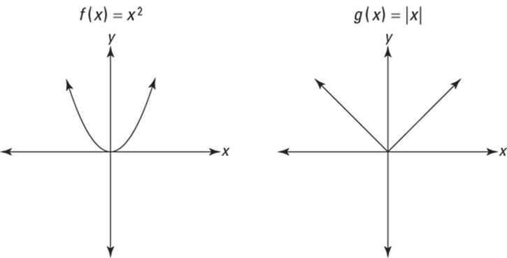
FIGURE 5-10: The graphs of ![]() and
and ![]()
Notice that both functions are symmetric with respect to the y-axis. In other words, the left and right sides of each graph are mirror images of each other. This makes them even functions. A polynomial function like ![]() where all powers of x are even, is one type of even function. (Such an even polynomial function can contain — but need not contain — a constant term like the 3 in the preceding function. This makes sense because 3 is the same as
where all powers of x are even, is one type of even function. (Such an even polynomial function can contain — but need not contain — a constant term like the 3 in the preceding function. This makes sense because 3 is the same as ![]() and zero is an even number.) Another even function is
and zero is an even number.) Another even function is ![]() (see Chapter 6).
(see Chapter 6).
A couple oddball functions
Graph ![]() and
and ![]() on your graphing calculator. These two functions illustrate odd symmetry. Odd functions are symmetric with respect to the origin which means that if you were to rotate them 180° about the origin, they would land on themselves. A polynomial function like
on your graphing calculator. These two functions illustrate odd symmetry. Odd functions are symmetric with respect to the origin which means that if you were to rotate them 180° about the origin, they would land on themselves. A polynomial function like ![]() where all powers of x are odd, is one type of odd function. (Unlike an even polynomial function, an odd polynomial function cannot contain a constant term.) Another odd function is y = sin(x) (see Chapter 6).
where all powers of x are odd, is one type of odd function. (Unlike an even polynomial function, an odd polynomial function cannot contain a constant term.) Another odd function is y = sin(x) (see Chapter 6).
Many functions are neither even nor odd, for example ![]() . My high school English teacher said a paragraph should never have just one sentence, so voilà, now it’s got two.
. My high school English teacher said a paragraph should never have just one sentence, so voilà, now it’s got two.
Exponential functions
An exponential function is one with a power that contains a variable, such as ![]() or
or ![]() . Figure 5-11 shows the graphs of both these functions on the same x-y coordinate system.
. Figure 5-11 shows the graphs of both these functions on the same x-y coordinate system.
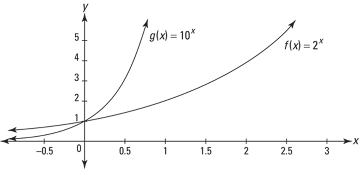
FIGURE 5-11: The graphs of ![]() and
and ![]() .
.
Both functions go through the point ![]() as do all exponential functions of the form
as do all exponential functions of the form ![]() . When b is greater than 1, you have exponential growth. All such functions get higher and higher without limit as they go to the right toward positive infinity. As they go to the left toward negative infinity, they crawl along the x-axis, always getting closer to the axis, but never touching it. You use these and related functions for figuring things like investments, inflation, and growing population.
. When b is greater than 1, you have exponential growth. All such functions get higher and higher without limit as they go to the right toward positive infinity. As they go to the left toward negative infinity, they crawl along the x-axis, always getting closer to the axis, but never touching it. You use these and related functions for figuring things like investments, inflation, and growing population.
When b is between 0 and 1, you have an exponential decay function. The graphs of such functions are like exponential growth functions in reverse. Exponential decay functions also cross the y-axis at ![]() , but they go up to the left forever, and crawl along the x-axis to the right. These functions model things that shrink over time, such as the radioactive decay of uranium.
, but they go up to the left forever, and crawl along the x-axis to the right. These functions model things that shrink over time, such as the radioactive decay of uranium.
Logarithmic functions
A logarithmic function is simply an exponential function with the x- and y-axes switched. In other words, the up-and-down direction on an exponential graph corresponds to the right-and-left direction on a logarithmic graph, and the right-and-left direction on an exponential graph corresponds to the up-and-down direction on a logarithmic graph. (If you want a refresher on logs, see Chapter 4.) You can see this relationship in Figure 5-12, in which both ![]() and
and ![]() are graphed on the same set of axes.
are graphed on the same set of axes.
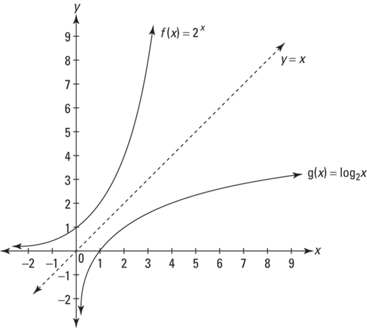
FIGURE 5-12: The graphs of ![]() and
and ![]()
Both exponential and logarithmic functions are monotonic. A monotonic function either goes up over its entire domain (called an increasing function) or goes down over its whole domain (a decreasing function). (I’m assuming here — as is almost always the case — that the motion along the function is from left to right.)
Notice the symmetry of the two functions in Figure 5-12 about the line ![]() . This makes them inverses of each other, which brings us to the next topic.
. This makes them inverses of each other, which brings us to the next topic.
Inverse Functions
The function ![]() and the function
and the function ![]() (read as “f inverse of x”) are inverse functions because each undoes what the other does. In other words,
(read as “f inverse of x”) are inverse functions because each undoes what the other does. In other words, ![]() takes an input of, say, 3 and produces an output of 9 (because
takes an input of, say, 3 and produces an output of 9 (because ![]() );
); ![]() takes the 9 and turns it back into the 3 (because
takes the 9 and turns it back into the 3 (because ![]() ). Notice that
). Notice that ![]() and
and ![]() . You can write all of this in one step as
. You can write all of this in one step as ![]() . It works the same way if you start with
. It works the same way if you start with ![]()
![]() (because
(because ![]() ), and
), and ![]() (because
(because ![]() ). If you write this in one step, you get
). If you write this in one step, you get ![]() . (Note that while only
. (Note that while only ![]() is read as f inverse of x, both functions are inverses of each other.)
is read as f inverse of x, both functions are inverses of each other.)
 The inverse function rule: The fancy way of summing up all of this is to say that
 ![]() and
and ![]() are inverse functions if and only if
are inverse functions if and only if ![]() and
and ![]() .
.
 Don’t confuse the superscript
 ![]() in
in ![]() with the exponent
with the exponent ![]() . The exponent
. The exponent ![]() gives you the reciprocal of something, for example
gives you the reciprocal of something, for example ![]() . But
. But ![]() is the inverse of
is the inverse of ![]() . It does not equal
. It does not equal ![]() , which is the reciprocal of
, which is the reciprocal of ![]() . So why is the exact same symbol used for two different things? Beats me.
. So why is the exact same symbol used for two different things? Beats me.
When you graph inverse functions, each is the mirror image of the other, reflected over the line ![]() . Look at Figure 5-13, which graphs the inverse functions
. Look at Figure 5-13, which graphs the inverse functions ![]() and
and ![]() .
.
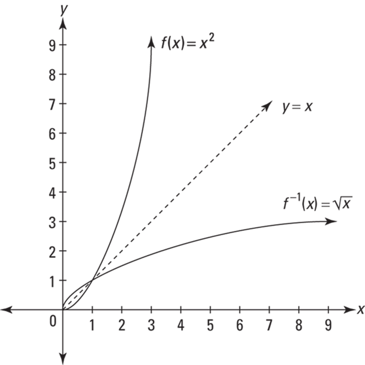
FIGURE 5-13: The graphs of ![]()
![]() and
and ![]()
If you rotate the graph in Figure 5-13 counterclockwise so that the line ![]() is vertical, you can easily see that
is vertical, you can easily see that ![]() and
and ![]() are mirror images of each other. One consequence of this symmetry is that if a point like
are mirror images of each other. One consequence of this symmetry is that if a point like ![]() is on one of the functions, the point
is on one of the functions, the point ![]() will be on the other. Also, the domain of f is the range of
will be on the other. Also, the domain of f is the range of ![]() , and the range of f is the domain of
, and the range of f is the domain of ![]() .
.
Shifts, Reflections, Stretches, and Shrinks
Any function can be transformed into a related function by shifting it horizontally or vertically, flipping it over horizontally or vertically, or stretching or shrinking it horizontally or vertically. I do the horizontal transformations first. Consider the exponential function ![]() . See Figure 5-14.
. See Figure 5-14.
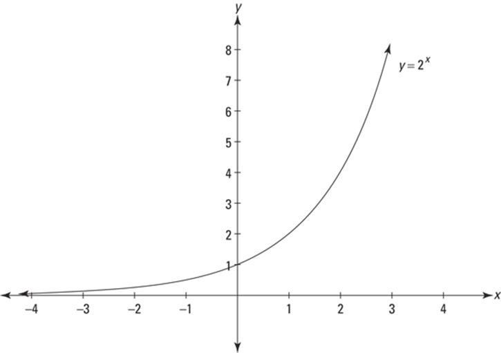
FIGURE 5-14: The graph of ![]()
Horizontal transformations
Horizontal changes are made by adding a number to or subtracting a number from the input variable x or by multiplying x by some number. All horizontal transformations, except reflection, work the opposite way you’d expect: Adding to x makes the function go left, subtracting from x makes the function go right, multiplying x by a number greater than 1 shrinks the function, and multiplying x by a number less than 1 expands the function. For example, the graph of ![]() has the same shape and orientation as the graph in Figure 5-14; it’s just shifted three units to the left. Instead of passing through
has the same shape and orientation as the graph in Figure 5-14; it’s just shifted three units to the left. Instead of passing through ![]() and
and ![]() , the shifted function goes through
, the shifted function goes through ![]() and
and ![]() . And the graph of
. And the graph of ![]() is three units to the right of
is three units to the right of ![]() . The original function and both transformations are shown in Figure 5-15.
. The original function and both transformations are shown in Figure 5-15.
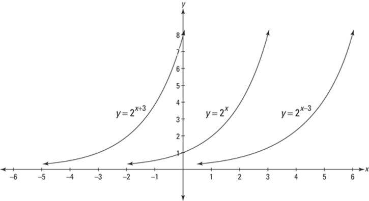
FIGURE 5-15: The graphs of ![]()
![]() and
and ![]()
If you multiply the x in ![]() by 2, the function shrinks horizontally by a factor of 2. So every point on the new function is half of its original distance from the y-axis. The y-coordinate of every point stays the same; the x-coordinate is cut in half. For example,
by 2, the function shrinks horizontally by a factor of 2. So every point on the new function is half of its original distance from the y-axis. The y-coordinate of every point stays the same; the x-coordinate is cut in half. For example, ![]() goes through
goes through ![]() , so
, so ![]() goes through
goes through ![]() ;
; ![]() goes through
goes through ![]() , so
, so ![]() goes through
goes through ![]() Multiplying x by a number less than 1 has the opposite effect. When
Multiplying x by a number less than 1 has the opposite effect. When ![]() is transformed into
is transformed into ![]() , every point on
, every point on ![]() is pulled away from the y-axis to a distance 4 times what it was. To visualize the graph of
is pulled away from the y-axis to a distance 4 times what it was. To visualize the graph of ![]() , imagine you’ve got the graph of
, imagine you’ve got the graph of ![]() on an elastic coordinate system. Grab the coordinate system on the left and right and stretch it by a factor of 4, pulling everything away from the y-axis, but keeping the y-axis in the center. Now you’ve got the graph of
on an elastic coordinate system. Grab the coordinate system on the left and right and stretch it by a factor of 4, pulling everything away from the y-axis, but keeping the y-axis in the center. Now you’ve got the graph of ![]() . Check these transformations out on your graphing calculator.
. Check these transformations out on your graphing calculator.
The last horizontal transformation is a reflection over the y-axis. Multiplying the x in ![]() by
by ![]() reflects it over or flips it over the y-axis. For instance, the point
reflects it over or flips it over the y-axis. For instance, the point ![]() becomes
becomes ![]() and
and ![]() becomes
becomes ![]() . See Figure 5-16.
. See Figure 5-16.
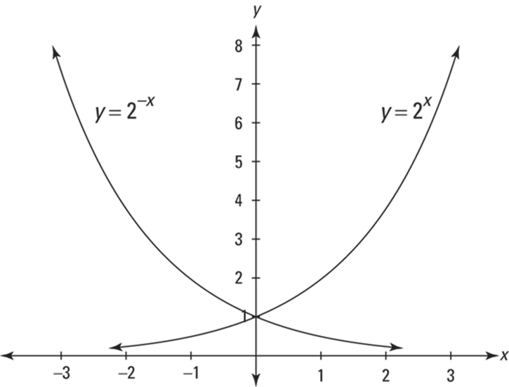
FIGURE 5-16: The graphs of ![]() and
and ![]()
Vertical transformations
To transform a function vertically, you add a number to or subtract a number from the entire function or multiply the whole function by a number. To do something to an entire function, say ![]() , imagine that the entire right side of the equation is inside parentheses, like
, imagine that the entire right side of the equation is inside parentheses, like ![]() . Now, all vertical transformations are made by placing a number somewhere on the right side of the equation outside the parentheses. (Often, you don’t actually need the parentheses, but sometimes you do.) Unlike horizontal transformations, vertical transformations work the way you expect: Adding makes the function go up, subtracting makes it go down, multiplying by a number greater than 1 stretches the function, and multiplying by a number less than 1 shrinks the function. For example, consider the following transformations of the function
. Now, all vertical transformations are made by placing a number somewhere on the right side of the equation outside the parentheses. (Often, you don’t actually need the parentheses, but sometimes you do.) Unlike horizontal transformations, vertical transformations work the way you expect: Adding makes the function go up, subtracting makes it go down, multiplying by a number greater than 1 stretches the function, and multiplying by a number less than 1 shrinks the function. For example, consider the following transformations of the function ![]() :
:
· ![]() shifts the original function up 6 units.
shifts the original function up 6 units.
· ![]() shifts the original function down 2 units.
shifts the original function down 2 units.
· ![]() stretches the original function vertically by a factor of 5.
stretches the original function vertically by a factor of 5.
· ![]() shrinks the original function vertically by a factor of 3.
shrinks the original function vertically by a factor of 3.
Multiplying the function by ![]() reflects it over the x-axis, or, in other words, flips it upside down. Look at these transformations on your graphing calculator.
reflects it over the x-axis, or, in other words, flips it upside down. Look at these transformations on your graphing calculator.
As you saw in the previous section, horizontal transformations change only the x-coordinates of points, leaving the y-coordinates unchanged. Conversely, vertical transformations change only the y-coordinates of points, leaving the x-coordinates unchanged.