The Calculus Primer (2011)

Part XIV. The Definite Integral

Chapter 52. INTEGRATION BETWEEN LIMITS

14—1. Generating an Area. Consider the shaded area “under” the curve y = ø (x) that is, the area RSMP, bounded by the ordinates SR and MP, by part of the X-axis, SM, and by the arc RP of the curve AB, or y = ø(x). This area may be considered as having been generated by a variable ordinate moving from an initial position of SR to a terminal position MP. If we represent this variable area by u, then it is clear that u is a function of x, and that u = 0 when x = a.

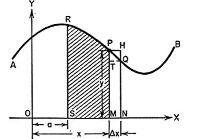
Now if we let x take on a small increment Δx, the area u takes on an increment Δu, or the area PMNQ. It is clear that, in the rectangles concerned,

area MNQT < area PMNQ < area MNHP

or, NQ·Δx < Δu< MP·Δx;

dividing by Δx:

As Δx → 0, MP remains constant and NQ → MP as a limit. Hence

or, in differential notation,

du = y dx. [1]

This equation may be stated as a general principle:

The differential of the area bounded by any curve, the X-axis, and two ordinates, is equal to the product of the ordinate which terminates the area and the differential of the corresponding abscissa.

14—2. The Definite Integral and Its Meaning. From the preceding paragraph, we have

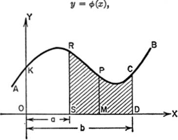
and du = y dx; hence du = ø(x) dx, where du represents the differential of the area between the curve y = ø(x), the X-axis, and any two ordinates such as SR and DC. Integrating the last equation, we have

u = ø (x) dx (1)

Since the expression ø(x) dx is a function of x, we may designate it as f(x) + C; thus

u = f(x) + C. (2)

It is possible to determine the value of C if we know the value of u for some value of x, as follows.

Let us arbitrarily begin to measure the area from the Y-axis.

Then:

when x = a, u = area OSRK;

when x = b, u = area ODCK;

hence, if x = 0, u = 0. Substituting in (2):

u = f(0) + C, or C = –f(0). (3)

Then equation (2) yields, by substituting (3) in (2):

u = f(x) – f(0). (4)

But equation (4) is a general expression for the area from the Y-axis to any ordinate, such as MP. So, to find the area between two particular ordinates, say SR and DC, we proceed as follows, substituting the appropriate abscissa for x in (4):

Area OSRK = f(a) – f(0) (5)

Area ODCK = f(b) – f(0) (6)

Subtracting equation (5) from (6):

Area SDCR = f(b) − f(a). (7)

14—3. Limits of Integration. The difference of the values of y dx for x = a and for x = b, as found in equation (7) of the preceding paragraph, is called “the integral from a to b of y dx.” It is represented by the symbol

It is called a definite integral, since its value is always definite, depending, of course, upon the values of a and b, as well as upon the nature of the function y dx. The process of finding the value of a definite integral is called “integrating between limits”; the value a is referred to as the lower limit, and b as the upper limit.

The reasoning of the previous paragraph may now be summarized symbolically as follows:

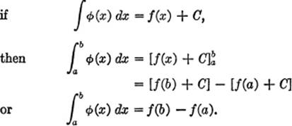
Although the expression as we have just seen, represents a definite area, the numerical value of the definite integral, namely, f(b) − f(a) may represent some quantity other than an area, or just a number, depending upon the problem from which the integral arises.

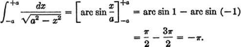
14—4. Calculating the Value of a Definite Integral. To find the numerical value of a definite integral, therefore, we first find the indefinite integral of the given differential; then, in this indefinite integral, we simply substitute for the variable first the upper limit and then the lower limit, and subtract the latter from the former. The procedure is illustrated in the following examples.

EXAMPLE 1. Find

Solution.

EXAMPLE 2. Find

Solution.

EXAMPLE 3. Find

Solution.

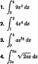
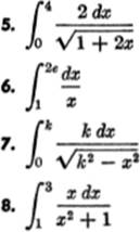
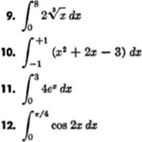
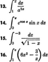
EXERCISE 14—1

Find the value of each of the following definite integrals: