Discrete Fractional Calculus (2015)
1. Basic Difference Calculus
1.7. First Order Linear Difference Equations
In this section we show how to solve the first order linear equation
![]()
(1.28)
where we assume ![]() and p(t) ≠ − 1 for
and p(t) ≠ − 1 for ![]()
We will use the following Leibniz formula to find a variation of constants formula for (1.28).
Theorem 1.67 (Leibniz Formula).
Assume ![]() . Then
. Then
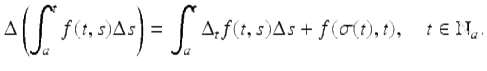
(1.29)
Proof.
We have that
![$$\displaystyle\begin{array}{rcl} \Delta \left (\int _{a}^{t}f(t,s)\Delta s\right )& =& \int _{ a}^{t+1}f(t + 1,s)\Delta s -\int _{ a}^{t}f(t,s)\Delta s {}\\ & =& \int _{a}^{t}[f(t + 1,s) - f(t,s)]\Delta s +\int _{ t}^{t+1}f(t + 1,s)\Delta s {}\\ & =& \int _{a}^{t}\Delta _{ t}f(t,s)\Delta s +\int _{ t}^{t+1}f(t + 1,s)\Delta s {}\\ & =& \int _{a}^{t}\Delta _{ t}f(t,s)\Delta s + f(\sigma (t),t), {}\\ \end{array}$$](fractional.files/image461.png)
which completes the proof. □
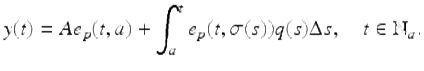
Theorem 1.68 (Variation of Constants Formula).
Assume ![]() and
and ![]() . Then the unique solution of the IVP
. Then the unique solution of the IVP

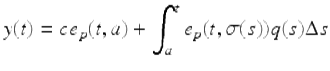
is given by
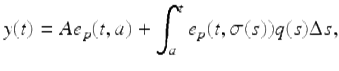
for ![]()
Proof.
The proof (see Exercise 1.56) of the uniqueness of solutions of IVPs for this case is similar to the proof of Theorem 1.29. Let
Using the Leibniz formula (1.29), we get
![$$\displaystyle\begin{array}{rcl} \Delta y(t)& =& Ap(t)e_{p}(t,a) +\int _{ a}^{t}p(t)e_{ p}(t,\sigma (s))q(s)\Delta s + e_{p}(\sigma (t),\sigma (t))q(t) {}\\ & =& p(t)\left [Ae_{p}(t,a) +\int _{ a}^{t}e_{ p}(t,\sigma (s))q(s)\Delta s\right ] + q(t) {}\\ & =& p(t)y(t) + q(t). {}\\ \end{array}$$](fractional.files/image467.png)
Also y(a) = A. □
Of course, it is always possible to compute solutions of difference equations by direct step by step computation from the difference equation. We next give an interesting example due to Gautschi [87] (and appearing in Kelley and Peterson [134, 135]) that illustrates that round off error can be a serious problem.
Example 1.69 (Gautschi [87]).
First we solve the IVP

Note that p(t): = t − 1 is a regressive function on ![]() . Using the variation of constants formula in Theorem 1.68, we get that the solution of our given IVP is given by
. Using the variation of constants formula in Theorem 1.68, we get that the solution of our given IVP is given by
![$$\displaystyle\begin{array}{rcl} y(t)& =& (1 - e)e_{t-1}(t,1) +\int _{ 1}^{t}e_{ t-1}(t,\sigma (s)) \cdot 1\Delta s {}\\ & =& e_{t-1}(t,1)\left [1 - e +\int _{ 1}^{t}e_{ t-1}(1,\sigma (s))\Delta s\right ] {}\\ & =& e_{t-1}(t,1)\left [1 - e +\int _{ 1}^{t} \frac{1} {e_{t-1}(\sigma (s),1)}\Delta s\right ]. {}\\ \end{array}$$](fractional.files/image470.png)
From Example 1.13, we have that e t−1(t, 1) = (t − 1)! . Hence
![$$\displaystyle\begin{array}{rcl} y(t)& =& (t - 1)!\left [1 - e +\int _{ 1}^{t} \frac{1} {(\sigma (s) - 1)!}\Delta s\right ] {}\\ & =& (t - 1)!\left [1 - e +\sum _{ s=1}^{t-1} \frac{1} {s!}\right ] {}\\ & =& -(t - 1)!\sum _{k=t}^{\infty }\frac{1} {k!}. {}\\ \end{array}$$](fractional.files/image471.png)
Note that this solution is negative on ![]() . Now if one was to approximate the initial value 1 − e in this IVP by a finite decimal expansion, it can be shown that the solution z(t) of this new IVP satisfies
. Now if one was to approximate the initial value 1 − e in this IVP by a finite decimal expansion, it can be shown that the solution z(t) of this new IVP satisfies ![]() and hence z(t) is not a good approximation for the actual solution. For example, if z(t) solves the IVP
and hence z(t) is not a good approximation for the actual solution. For example, if z(t) solves the IVP
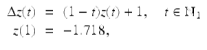
then z(2) = −. 718, z(3) = −. 436, z(4) = −. 308, z(5) = −. 232, z(6) = −. 16, z(7) = . 04 and after that z(t) increases rapidly with ![]() Hence z(t) is not a good approximation to the actual solution y(t) of our original IVP.
Hence z(t) is not a good approximation to the actual solution y(t) of our original IVP.
A general solution of the linear equation (1.28) is given by adding a general solution of the corresponding homogeneous equation ![]() to a particular solution to the nonhomogeneous difference equation (1.28). Hence by Theorem 1.14 and Theorem 1.68
to a particular solution to the nonhomogeneous difference equation (1.28). Hence by Theorem 1.14 and Theorem 1.68
is a general solution of (1.28). We use this fact in the following example.
Example 1.70.
Find a general solution of the linear difference equation
![]()
(1.30)
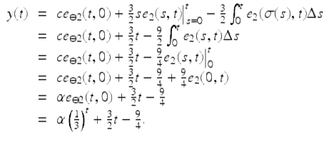
Note that the constant function ⊖ 2 is a regressive function on ![]() . The general solution of (1.30) is given by
. The general solution of (1.30) is given by
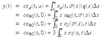
Integrating by parts we get