Discrete Fractional Calculus (2015)
1. Basic Difference Calculus
1.6. Discrete Taylor’s Theorem
In this section we want to prove the discrete version of Taylor’s Theorem. First we study the discrete (delta) Taylor monomials and give some of their properties. We will see that these discrete Taylor monomials will appear in the discrete Taylor’s Theorem. These (delta) Taylor monomials take the place of the Taylor monomials ![]() in the continuous calculus.
in the continuous calculus.
Definition 1.60.
We define the discrete Taylor monomials (based at ![]() ), h n (t, s),
), h n (t, s), ![]() by
by
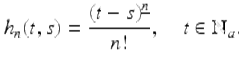
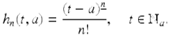
In particular if s = a, then
Theorem 1.61.
The Taylor monomials satisfy the following:
(i)
![]()
(ii)
![]()
(iii)
![]()
(iv)
![]()
(v)
![]()
(vi)
![]()
where C is a constant.
Proof.
We will only prove part (v). Since
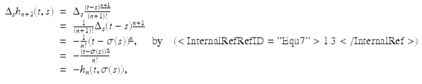
we have that (v) holds. □
Now we state and prove the discrete Taylor’s Theorem.
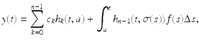
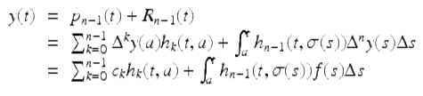
Theorem 1.62 (Taylor’s Formula).
Assume ![]() and
and ![]() . Then
. Then
![]()
where the n-th degree Taylor polynomial, p n (t), is given by
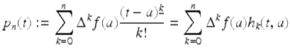
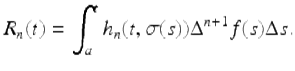
and the Taylor remainder, R n (t), is given by
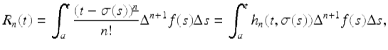
for ![]()
Proof.
If n = 0, then
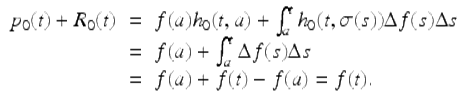
Hence Taylor’s Theorem holds for n = 0. Now assume that n ≥ 1. We will apply the second integration by parts formula in Theorem 1.58, namely (1.27), to
To do this we set
![]()
then it follows that
![]()
Using Theorem 1.61, (v), we get
![]()
Hence we get from the integration by parts formula (1.27), that
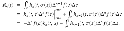
If n ≥ 2, then again we apply the integration by parts formula (1.27), to get
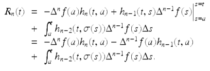
By induction on n, we get
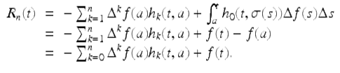
Solving for f(t) we get the desired result. □
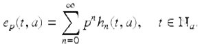
Definition 1.63.
If ![]() , then we call
, then we call
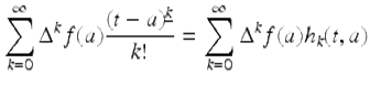
the (formal) Taylor series of f based t = a.
The following theorem gives us some Taylor series for various functions.
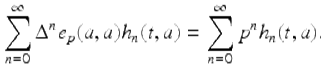
Theorem 1.64.
Assume p is a constant. Then the following hold:
(i)
If p ≠ − 1, then ![]()
(ii)
If p ≠ ± 1, then ![]()
(iii)
If p ≠ ± 1, then ![]()
(iv)
If p ≠ ± i, then ![]()
(v)
If p ≠ ± i, then ![]()
for all ![]()
Proof.
We first prove part (i). Since ![]() for each
for each ![]() we have that the Taylor series for e p (t, a) is given by
we have that the Taylor series for e p (t, a) is given by
To show that the above Taylor series converges to e p (t, a), for each ![]() , it suffices to show that the remainder term, R n (t), in Taylor’s formula, satisfies
, it suffices to show that the remainder term, R n (t), in Taylor’s formula, satisfies
![]()
for each fixed ![]() .
.
So fix ![]() and consider
and consider
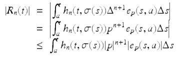
Since t is fixed, there is a constant C such that
![]()
Hence
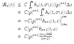
Since (t − a) n+1 = 0, for n ≥ t − a, we have that R n (t) = 0 for n ≥ t − a, so for each fixed t, ![]() Hence,
Hence,
To see that (ii) holds for ![]() , note that for p ≠ ± 1
, note that for p ≠ ± 1
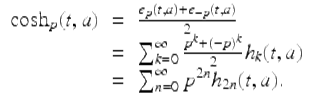
Similarly, since ![]()
![]() , and
, and ![]() , are defined in terms of exponential functions, parts (iii)–(v) follow easily from part (i). □
, are defined in terms of exponential functions, parts (iii)–(v) follow easily from part (i). □
We next show that Taylor’s Theorem gives us a variation of constants formula.
Theorem 1.65 (Variation of Constants Formula).
Assume ![]() . Then the unique solution of the IVP
. Then the unique solution of the IVP
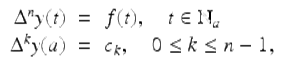
where c k , 0 ≤ k ≤ n − 1, are given constants is given by
for ![]()
Proof.
The proof of uniqueness is similar to the proof of Theorem 1.29. Using Taylor’s Theorem 1.62, we get the solution, y(t), of the given IVP is given by
for ![]() □
□
We now give a very elementary example to illustrate the variation of constants formula.
Example 1.66.
Use the integer variation of constants formula to solve the IVP
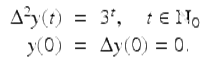
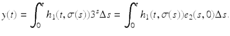
Using the variation of constants formula in Theorem 1.65, the solution of the given IVP is given by
Integrating by parts we get
![$$\displaystyle\begin{array}{rcl} & & y(t) = \frac{1} {2}(t - s)e_{2}(s,0)\vert _{s=0}^{t} + \frac{1} {2}\int _{0}^{t}e_{ 2}(s,0)\Delta s {}\\ & & = -\frac{1} {2}t + \frac{1} {4}[e_{2}(s,0)]_{s=0}^{t} {}\\ & & = -\frac{1} {2}t + \frac{1} {4}[e_{2}(t,0) - 1] {}\\ & & = -\frac{1} {2}t -\frac{1} {4} + \frac{1} {4}3^{t}, {}\\ \end{array}$$](fractional.files/image455.png)
for ![]() Of course one could easily solve the IVP in this example by twice integrating both sides of
Of course one could easily solve the IVP in this example by twice integrating both sides of ![]() from 0 to t (Exercise 1.52).
from 0 to t (Exercise 1.52).