Mathematics of Life (2011)

Chapter 4. Florally Finding Fibonacci

The first two revolutions in biology set the pattern of subsequent research for over a century. The accepted way to advance biological knowledge was to seek out new species and fit them into the Linnaean scheme; to study them in detail, using a microscope where necessary, and to record and report what you found. This was the ‘butterfly collecting’ era of biology, when the aim was to catalogue life’s diversity and celebrate its richness.

Amid the deluge of detail, a few general principles started to emerge, especially when it came to general relationships between organisms such as predator/prey, parasite/host, mimicry and symbiosis. These concepts helped to organise an ever-growing body of knowledge. But the predominant model was to collect, catalogue and observe. You weren’t a biologist: you were a botanist (specialising in plants), a zoologist (animals), an entomologist (insects), a herpetologist (snakes), an ichthyologist (fishes), and so on.

The physical sciences followed a very different path. The same period, from Linnaeus in 1735 to Darwin in 1859, witnessed the explosive growth of physics, fuelled by the discovery of universal laws of nature, expressed in the arcane language of mathematics. But while physics was being unified by general mathematical principles, biology was being overwhelmed by a morass of individual examples. There were few general principles, hardly any laws to speak of and virtually no mathematics.

Even so, mathematics managed to squeeze itself into a few areas of biology, notably the strange numerology of the plant kingdom. A very specific sequence of numbers shows up repeatedly in association with plants, in several different contexts: the number of petals in a flower, the geometry of seed heads, the arrangement of leaves along a stem, the lumps on a cauliflower, and the way pineapples and pine cones fit together.

With the mathematical techniques available and the view of biology that prevailed around 1850, these numerical patterns could be – and were – described in considerable detail. Description, though, was as far as it went. Explaining why the patterns occurred was another matter entirely, beyond the scope of the science of that period. In this chapter, we will see how far Victorian-era science managed to get when grappling with the numerology and geometry of plants. Then, temporarily diverting from the historical story, we’ll see how modern mathematics and a dash of chemistry have filled some of the gaps.

Marigolds typically have 13 petals. Asters have 21. Many daisies have 34 petals; if not, they usually have 55 or 89. Often, especially in cultivated plant varieties, the number of petals is twice as large, because plant breeders have learned how to double up the petals. On the whole, though, you seldom see a daisy with 37 petals, and if you see one with 33 then a petal has probably fallen off. Sunflowers, which also belong to the daisy family, usually have 55, 89 or 144 petals. Exceptions are usually the result of damage or disturbance while the young plant is maturing.

At first sight, there seems to be no particular reason why nature should favour these numbers – or any specific number, come to that. Petals are arranged like the spokes of a wheel around the central region of the flower. Just as a wheel can have any number of spokes, there seems to be no obvious restriction on how many petals can or cannot fit into the available space. This makes the limited list of numbers distinctly mysterious.

From today’s gene-centred viewpoint, a plant could presumably have any reasonable number of petals, depending on the ‘instructions’ coded in its genes. So we would expect to find specific numbers for particular species, but not the same small list of rather strange numbers for many different species. However, this is what nature supplies, as Table 2 (see over) indicates. Other numbers are much rarer, though they do occur: for example, fuchsias have 4 petals. Exceptions like this often involve the numbers 4, 7, 11, 18 and 29, and I’ll return to these later because they actually confirm more modern theories, rather than disproving them.

Table 2 The number of petals on a flower.

To compound the mystery, the same curious numbers show up elsewhere in the plant kingdom. A notable example is the arrangement of leaves on the stem of a plant, technically known as phyllotaxis. Some plants use very simple arrangements, with leaves arranged in pairs, one on either side. But many arrange their leaves in a helix, so that successive leaves along the stem are placed at a specific angle relative to the previous leaf. And those angles involve the same list of special numbers.

A typical case occurs for an angle of 135°, which is 3/8 of a full circle. If we say that the first leaf is at angle 0°, then the second will be at 135°, the third at 270°, and so on. The angles of successive leaves are the integer multiples of 135°. Subtracting 360° whenever the numbers become larger than a full turn, we obtain the sequence of angles (with the corresponding fractions of a full circle listed underneath):

This pattern then repeats indefinitely. (I’ve left fractions like 6/8 as they are instead of reducing them to 3/4 to make the pattern clearer.) Figure 7 shows how these angles create a helical arrangement of leaves.

The same kind of behaviour occurs for many other plants, but several different fractions of a full turn can occur. However, other simple fractions, such as 2/7, are conspicuously absent. The ones listed in Table 3 are closely related to the numbers observed in petals. In fact, each fraction in the list is formed from two of the numbers 1, 2, 3, 5, 8, 13. Apart from 1 and 2, these are all petal numbers. This is not a complete surprise, because petals are modified leaves, but it requires explanation.

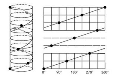
Fig 7 Left: The helical arrangement of successive leaves separated by 3/8 of a turn. Right: The same helix on the cylindrical surface of the plant stem rolled out flat. Note that 360° is equivalent to 0°, so the two ends ‘wrap round’ and join.

Table 3 Fractions of a turn between successive leaves in different plants.

Exactly the same numbers show up in several other features of plants, adding to the evidence that these patterns are not mere coincidence. Pineapples are easily recognised by the roughly hexagonal pattern on their surface. The hexagons are individual fruits, which coalesce as they grow. They fit neatly together, not into the standard honeycomb tiling, but into two interlocking families of helical spirals. One family winds anticlockwise, viewed from above, and contains 8 spirals; the other winds clockwise, and contains 13. It is also possible to see a third family of 5 spirals, winding clockwise at a shallower angle (Figure 8, see over). The scales of pine cones form similar sets of spirals. So do the seeds in the head of a ripe sunflower (Figure 9), but now the spirals are not helical, but lie in a plane.

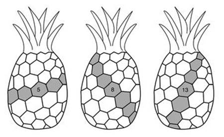
Fig 8 Three families of spirals in a pineapple.

Fig 9 Two families of spirals in the head of a sunflower: 34 wind clockwise, 21 anticlockwise.

Clearly there is something about this list of numbers that makes them unusually suitable for plant structure. But why are these numbers so common, while others are much rarer?

The answer began with rabbits.

In 1202 the Italian mathematician Leonardo of Pisa wrote a textbook on arithmetic. One of the exercises he set his readers was a problem about the progeny of a pair of rabbits. I’ll discuss this problem and its answer in more detail in Chapter 16, when we take a look at the mathematics of population growth. Here we need to focus only on the resulting sequence of numbers, which lists how many pairs of rabbits there are in successive breeding seasons:

and so on. The rule for forming these numbers (other than the first two 1’s, which we take as a starting point) is that each is obtained by adding the previous two: 2=1+1, 3=1+2, 5=2+3, 8=3+5, 13=5+8, and so on. Leonardo later acquired the nickname Fibonacci, and ever since 1877, when the French mathematician and populariser Édouard Lucas wrote about this sequence, its members have been known as the Fibonacci numbers.

To paraphrase J.B.S. Haldane, the plant kingdom seems to have an inordinate fondness for Fibonacci numbers.

Leonardo’s association of this sequence with rabbit progeny, though superficially biological, is completely irrelevant to petal numbers and phyllotaxis. Indeed, its assumptions are so artificial that it’s not terribly relevant to rabbits either. But one mathematical feature of the answer is distinctly relevant: the fractions formed by successive Fibonacci numbers. If we write these fractions as decimals, something emerges:

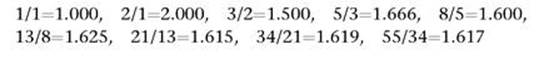
As the numbers increase, the fraction gets closer and closer to a particular value, which to six decimal places is 1.618034. In fact, it is exactly equal to (1+√5)/2, and is usually denoted by the symbol φ (the Greek letter phi). This number is irrational: that is, it cannot be represented by the ratio of two integers – no fraction can be exactly equal to it. In fact, it was one of the earliest irrational numbers discovered, after the square root of two, and it was known to the ancient Greeks in the context of the geometry of pentagons.

The fractions that appear in phyllotaxis are also ratios of Fibonacci numbers, but instead of using consecutive members of the sequence, the numerator (top) and denominator (bottom) are spaced two steps apart. Moreover, the larger number is the denominator, not the numerator. A typical case is 5/13, constructed from the portion of the Fibonacci sequence that reads 5, 8, 13. The first few fractions of this type are:

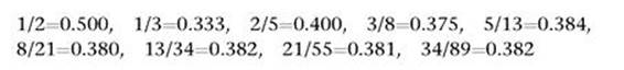
Again we see a pattern: the fractions get closer and closer to a particular number, this time 0.381966. This number is closely related to φ. In fact, some simple algebra shows that the exact value is 2-φ.

The special properties of the golden number φ provide an alternative interpretation. Suppose we divide a full circle (360°) into two arcs that are in golden ratio. That is, the angle determined by the larger arc is φ times the angle determined by the smaller arc. Then the smaller arc is 1/(1+φ) times a full circle. Numerically, this expression is 0.381966: the number derived above. A bit more algebra confirms that this relationship is exact. Numerically, this angle is very close to 137.5°, and it is called the golden angle.

The upshot of all this is that we can interpret the fractions observed in phyllotaxis as approximations to the golden angle. That’s all very well, but so far we have just replaced one mathematical puzzle by two others. The occurrence of Fibonacci numbers in flowers now seems to depend on a special angle and a sequence of related fractional approximations. Why this angle, and why these fractions?

The fractions are the easier part: they can be characterised mathematically as the best fractional approximations to the golden angle, for a given size of denominator. Not just in the sense that, say, 3/8 is a closer approximation than 2/8 or 4/8, but that if you look at fractions with larger denominators, the first time you get a closer approximation is when you reach 5/13. After that, the next improvement comes at 8/21, and so on. Classical mathematical concepts known as ‘continued fractions’ establish this relationship between the golden angle and the phyllotaxis fractions. So the key to the mystery is to understand why the golden angle appears. If we can do that, the role of the fractions should follow.

The next step in solving the riddle of phyllotaxis was biological: specifically, taking a look at how the shoot of a growing plant changes on the cellular level. In 1868 the German botanist Wilhelm Hofmeister made extensive observations of this process, and laid the foundations for all subsequent work on the problem.

In the early stage of development, a plant appears to be little more than a tiny green shoot, with little structure. As it grows, small leaves begin to appear, and are ‘left behind’ as the shoot heads skyward. The main changes occur at the tip of the shoot. We can get a reasonable mental image of the growth pattern by thinking of a fountain, where water sprays upwards from the centre, moves outward radially and then starts to fall back towards the surface of the pond. Now suppose that the entire fountain heads skywards like a rocket, and the water that trails behind it ‘freezes’ once it drops below the level of the fountain’s centre. Then you would see a growing column of frozen water, with a spurting fountain, climbing towards the heavens, perched precariously on top of it. All of the ‘new’ water would be produced by the fountain at the tip of the column, from which it would migrate radially until it reached the column’s edge and froze.

A growing shoot is like that, but using new cells in place of droplets of water. For simplicity we can think of the shoot as a cylinder with a rounded top. Most new growth occurs near the tip of the shoot, close to the centre of the stem. New cells appear, through cell division, near the centre of the tip, and they migrate outwards towards the edge, where (at this level of description) they stop. In this way the growing tip pushes upwards, leaving a trail of new cells behind it, and the cylindrical column becomes taller without getting thicker.

As the plant matures, of course, the stem does get thicker, and many other changes occur, such as leaves getting bigger, buds appearing, and so on. But the explanation of phyllotaxis does not depend on these later changes: the basic pattern of leaf development – and much else – is determined by what happens at the growing tip.

The events unfolding there would be invisible without a microscope, because they involve small clumps of cells known as primordia (plural of primordium). Each clump will eventually become a leaf, so the positions of the leaves are set by the microscopic geometry of the primordia. Hofmeister discovered that the process begins with the appearance of two primordia, located together at the centre of the tip, on opposite sides. As these two start to migrate radially outwards, a third primordium appears near the centre, between them. There is insufficient room for this new primordium to grow to full size in that location, and the previous two push it away from the centre into an open space. The interplay of these forces causes the three primordia to arrange themselves so that the angles between the first and second, and the second and third, are close to the golden angle.

Before these three primordia have moved very far, a fourth appears near the centre of the tip. Because three times the golden angle is a little bit more than a full turn of 360°, this fourth primordium appears close to the first one and pushes it outwards. Then a fifth appears near the centre, and pushes against the second, as shown in Figure 10. The result of all this pushing and shoving, with new primordia popping into existence in the middle while the others move slowly outwards, is a beautiful geometric pattern. Successive primordia are spaced at multiples of the golden angle along a spiral. The shape of the spiral is determined by the rate at which the primordia move, and grow, so Hofmeister called it the generative spiral.

Shorn of the biological detail, we now have a mathematical description of the process that creates the geometrical and numerical patterns in phyllotaxis. Successive primordia lie on the generative spiral, each separated from its successor by the golden angle or a close approximation to it. As time passes, any given primordium migrates radially until it reaches the edge of the stem’s rounded tip, at which point it stops moving. As the shoot grows, the result is a series of primordia, spaced at integer multiples of the golden angle along a helix that winds up the cylinder that represents the stem.

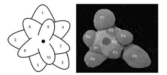
Fig 10 Left: Theory. Successive primordia (numbered in order of appearance) lie at a fixed angle to the previous one, and slowly migrate outwards. Right: Experiment. The growing tip of Arabidopsis (cress) as seen by an electron microscope, showing successive primordia (P8 – P1 – the numbers are in reverse order compared to the previous picture). The next primordium will appear at P0. The region surrounding P0 is the source of new cells.

Victorian mathematicians, among them the mathematical physicist Peter Guthrie Tait, best known for his Treatise on Natural Philosophy, turned Hofmeister’s ideas into a tidy mathematical description of phyllotaxis, based on diagrams like Figure 7 (see p. 41). But description was as far as Victorian mathematics got. At least one crucial question remained open: what is so special about the golden angle when it comes to plant growth? Yes, the golden angle comes from the golden number, but why is the golden number relevant?

In On Growth and Form, Thompson discusses one popular answer from the Victorian era: since the golden number is irrational, such an arrangement prevents any leaf from being exactly above another, allegedly allowing rain and sunlight to reach the leaves more effectively. He points out that the same argument works for any irrational number, and that the golden number can be obtained from many number sequences, not just the Fibonacci sequence. (He might also have pointed out that the approximations such as 5/13 that appear in real plants, which we are trying to explain, are rational.) He remarks, dismissively, that ‘all such speculations as these hark back to a school of mystical idealism’.

In 1917, when Thompson’s book first appeared, this must have seemed a shrewd comment. Golden numbers and Fibonacci sequences had a cultish appeal, and gave rise to an extensive literature that was long on speculation and short on fact. However, more recent work has established that the golden angle is a genuine feature of plant numerology, and so are its Fibonacci-fraction approximations. The reasons go beyond number mysticism by moving on from merely describing the geometry, and taking account of the dynamics of the growing plant. Progress on this problem has occurred in a series of steps, and we can take the story a little further here by temporarily following more modern developments, before returning to the historical order in the next chapter, with the third revolution in biology.

The special features of the golden angle are easier to appreciate if we turn to a related feature of plants: not the positioning of primordia as the young shoot first grows, but the positioning of seeds in the flower of a mature plant. Fibonacci numbers are to be found here as well. So is Hofmeister’s generative spiral, because the locations of the seeds are determined by patterns of primordia in the young shoot. These patterns are not activated until the plant matures, but they are created by the same mechanism that generates leaves. So again, the main issue is the geometry of primordia, which generate not only the leaves of the plant but many of the other interesting organs, including the petals, and the seeds in the seed-head.

We’ve already seen in Figure 9 (see p. 42) that the seeds in a sunflower head are packed together in such a way that the human eye is immediately attracted to two interpenetrating families of spirals, one running clockwise, the other anticlockwise. If you count how many spirals there are in each family, you typically find two consecutive Fibonacci numbers. By the way, these spirals are not the generative spiral, which is more loosely wound and not apparent to the eye – unless you join primordia in the order in which they form.

Petals form at the outer end of one family of spirals, again cryptically determined by the original pattern of primordia, which are specialised to form petals, not seeds. So a Fibonacci number of spirals implies a Fibonacci number of petals. In short, it is enough to explain why Fibonacci numbers turn up in the spirals.

In 1979, Helmut Vogel of the Technical University of Munich considered a simple mathematical representation of the geometry of sunflower seeds, and used it to explain why the golden angle is especially suited to such arrangements.¹ In his model, the nth primordium is placed at an angle equal to n times 137.5°, and its distance from the centre is proportional to the square root of n. These two numbers determine its location, and Hofmeister’s generative spiral is revealed as a so-called Fermat spiral, which becomes more tightly wound as it moves outwards from the centre.

Using this formula, Vogel worked out what would happen to the seed head if the same generative spiral were employed, but the golden angle of 137.5° were changed, ever so slightly. The result, shown in Figure 11, is striking. Only the golden angle leads to seeds that are packed closely together, with no gaps or overlaps. Even a change in the angle of one-tenth of a degree causes the pattern to break up into a single family of spirals, with gaps between the seeds.

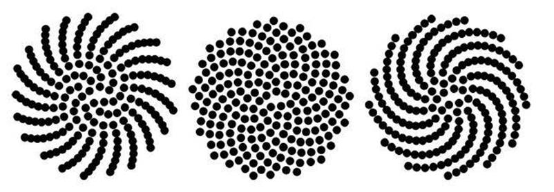
Fig 11 Fermat spiral patterns. Left: Spacing 137°, just less than the golden angle. Middle: Spacing 137.5°, the golden angle. Right: Spacing 138°, just greater than the golden angle.

Vogel’s model explains why the golden angle is special, and supports the view that it plays an active role in phyllotaxis, and is not some numerical coincidence viewed through mystical eyes. However, the full explanation lies deeper. It turns out that – just as Hofmeister had said – the dynamics of the growing plant causes primordia to be pushed into golden-angle relationships. As the cells grow and move, they create forces that affect neighbouring cells.

Forces are an essential ingredient of mechanics, which is the mathematical physics of moving objects. Mechanics was born in experiments that Galileo made around 1600, when he rolled balls down a slope to investigate the effects of gravity. It became a recognised branch of mathematics in 1687, when Newton published his epic Philosophiae Naturalis Principia Mathematica (‘Mathematical Principles of Natural Philosophy’) in which he related the motion of a body to the forces acting on it. It has since become a cornerstone of science.

Once mechanics enters the picture, attention switches from merely describing natural phenomena to investigating the mechanisms that cause them. The golden angle and its Fibonacci fractions cease to be numerical curiosities, and their presence is now explained by the interplay of forces in the growing stem. Contrary to Thompson’s scepticism, the golden number and the mathematics associated with it do, in fact, play key roles.

In 1992 the French mathematical physicists Stéphane Douady and Yves Couder investigated the mechanics of systems in which point-like objects representing primordia are repeatedly introduced near the centre of a circular disc at equally spaced instants of time, and then made to move outwards along a radius of the circle.² They assumed that these objects repel each other, much as two north poles of magnets do. Then they worked out what would happen in two ways: by experiment, and by computer simulation.

In their experiments, successive primordia were represented by droplets of magnetic fluid, under the action of a magnetic field that caused them to repel each other, so that they organised one another into patterns while migrating in a radial direction. The result depended on the strength of the magnetic field and the intervals between droplets, but in the most common pattern that developed the droplets spontaneously packed themselves into families of spirals just like those in the sunflower head, complete with golden angle and Fibonacci numerology.

Computer simulations revealed more detail, showing that the system of droplets naturally homes in on Fibonacci-fraction approximations to the golden angle. The fraction that emerges depends on the rate at which new droplets are added. The precise relation is captured by a so-called bifurcation diagram (Figure 12). This shows how the numbers in the spirals, and the associated angle between successive primordia, relate to this rate. The main features of the bifurcation diagram are two curves, called the Fibonacci branch and the Lucas branch. There are other branches – in principle infinitely many – but these are very short, so they rarely occur in practice.

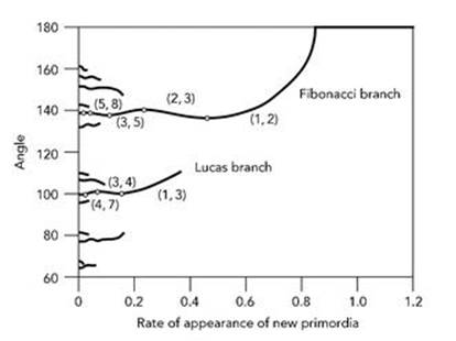
Fig 12 Bifurcation diagram for phyllotaxis, after Douady and Couder.

To interpret the curves, we start at the right hand end and move to the left. When the rate of droplet formation is bigger than 0.8, the angle is 180°, so successive droplets line up on either side of the centre. As the rate slows down, the angle changes continuously, following the curve that bends from the top of the picture down towards the left, and the angle changes to about 140°. This curve, the Fibonacci branch, corresponds to the most likely behaviour. It wiggles up and down, and at each peak or trough (shown by a white dot) the numbers of spirals in the two families move one step up the sequence. If we write, say (3, 5) to mean 3 families in one direction and 5 in the other, then these pairs of numbers change from (1, 2) to (2, 3), then to (3, 5), then to (5, 8), and so on, as the curve runs from right to left. The angle converges towards the golden angle of 137.5°, as expected.

Now the remaining pieces of the mathematical puzzle were falling into place: why the golden angle is the organising principle behind the geometry, and why what we actually observe are Fibonacci-fraction approximations. The main missing ingredient was a rigorous mathematical proof that the features seen in the simulations are what they appear to be. This was provided in 1991 by Leonid Levitov, a condensed matter physicist now at the Massachusetts Institute of Technology. In 1995 Martin Kunz, a physicist at the University of Lausanne in Switzerland, added many further details.³

These results also explained a puzzling feature of the problem which I have glossed over so far: the occasional appearance of non-Fibonacci numbers, such as the four petals of the fuchsia. These exceptions also appear in Douady and Couder’s bifurcation diagram, but on the Lucas branch – so they have the same explanation as the Fibonacci numbers. Now the numbers of spirals come from a sequence very like the Fibonacci sequence, called the Lucas numbers:

and so on. The rule for forming the numbers, after the first two, is the same as before: each number is the sum of the previous two, but here the first two numbers are 1 and 3, not 1 and 1. The ratios of successive Lucas numbers also approach the golden number. The pairs of numbers of spirals now become (1, 3), then (3, 4), then (4, 7), then (7, 11), and so on. The angle converges to 99.5°.

The other, shorter, branches in the bifurcation diagram correspond to patterns that follow sequences like the Fibonacci and Lucas sequences, but starting with different numbers. They correspond to angles such as 77.9° and 151.1°, and are hardly ever seen in plants.

The four petals of the fuchsia are not the only occurrence of Lucas numbers in plants. Some cacti exhibit a pattern of 4 spirals in one direction and 7 in the other, or 11 in one direction and 18 in the other. A species of echinocactus has 29 ribs.⁴ Sets of 47 and 76 spirals have been found in sunflowers.⁵

Cacti lead naturally to an extension of the mathematical analysis of plant structure. In the models I have just described, primordia are represented as discrete point-like objects, and the forces act on the associated points. In a more realistic ‘continuum’ model, the forces would be distributed over the entire surface of the growing stem, and the primordia would develop as a consequence of those forces, much as a sheet of metal will buckle when its edges are compressed. The techniques required here come from a major branch of applied mathematics: elasticity theory. This studies how shapes that are able to bend or compress behave when they are subjected to external forces; it is widely used by engineers when designing buildings, bridges and other large structures.

If you distort an elastic object, you have to do work. Think of squeezing a rubber ball, for instance. The work you do in squeezing the ball is stored in the material as a form of energy, known as elastic energy. A central principle in elasticity theory is that systems behave so as to minimise their elastic energy. In 2004, Patrick Shipman and Alan Newell, mathematicians at the University of Arizona in Tucson, applied elasticity theory to continuum models of a growing plant shoot, with particular emphasis on cacti – which are widespread in Arizona.⁶ They modelled the formation of primordia as a kind of buckling of the surface of the tip of the growing shoot, and showed that minimum-energy configurations take the form of superimposed patterns of parallel waves.

These patterns are governed by two factors: the wave number, which is related to wavelength, and the direction in which the waves point. The Fibonacci numerology, in this approach, arises because the most important patterns involve the interaction of three such waves, and in the relevant states, the wave number for the third wave must be the sum of the other two wave numbers. The spirals on the pineapple in Figure 8 (see p. 42) show three systems of roughly parallel lines of hexagons: it’s basically the same idea. So this model traces the arithmetic of Fibonacci numbers directly to the arithmetic of wave patterns. Not only the numbers, but even the mathematical rule for their formation, correspond directly to the underlying mechanics of the buckling tip.

Any botanist will tell you that plant tips don’t really buckle: they grow. So although the elasticity model captured some of the main features of plant growth, it was still missing some crucial ingredient. The forces that act on primordia explain their geometry, but they don’t explain how new primordia are produced, and why they appear at the places where elastic buckling says they should.

The answer to this question required not mathematics, but biochemistry. The formation of primordia is driven by a hormone, called auxin. Newell and colleagues have shown that similar wave patterns arise in the auxin distribution.⁷ So the story as it is now understood involves an interplay among the biochemistry of the growing plant, the mechanical forces between cells, and the plant’s geometry. Auxin stimulates the growth of new primordia. Primordia exert forces on one another and, in combination with the growth of the plant, these forces create the geometry. The geometry may also affect the plant’s biochemistry, for example by triggering the production of extra auxin in specific places. So there is a complex set of feedback loops between biochemistry and mechanics, mechanics and geometry, and geometry and biochemistry – and all of these ingredients are required. Current mathematical theories therefore have to take into account many features of the biology and physics of the growing plant that were undreamt of in Victorian times.

As a result of all this activity, we now know that D’Arcy Thompson’s scepticism was unfounded. The role of the golden number in phyllotaxis is genuine and informative. The associated mathematics provides a convincing explanation – indeed, several complementary ones – of Fibonacci numerology. It also explains why some plants do not have Fibonacci numbers of petals, by predicting the rarer occurrence of Lucas numbers. These account for most of the exceptions seen in nature. So the Victorian work on the golden angle, as a description of phyllotaxis, has motivated deeper mathematical theories that are more broadly applicable. What seemed to be exceptions, a century ago, actually confirm the deeper mathematical theory that underpins the Victorian one.

However, many plants do not fit into even this more general description of phyllotaxis. Some even seem to produce leaves and other organs pretty much at random. So the story is still incomplete.

A word of warning is also in order. Thompson had a reason for his doubts, and it has not entirely gone away. Humanity’s fascination with the golden number has often led to exaggerated claims for its importance, usually in contexts that are mathematically vague. Entire books have been written about the golden number in nature and art, finding it in the spirals in goats’ horns and in the proportions of the Great Pyramid and the Parthenon. It is often stated that the most aesthetically pleasing shape for a rectangle occurs when its sides are in the golden ratio.

There seems to be very little basis for this claim: it is a mathematical urban myth. Many of these supposed occurrences of golden numerology are probably spurious or accidental. Some methods of statistical analysis can concentrate data around the golden number, exaggerating its significance. Any measurement close to 1.6 can be attributed to the golden number, but the relationship is likely to be coincidental, unless – as is now known to be the case for phyllotaxis – the phenomenon concerned arises from a deeper model in which the golden number turns up for solid structural reasons.

It is also often stated that the nautilus shell, which forms a beautiful spiral, is an example of the golden number in nature. This is a misunderstanding. The shape of the shell is impressively similar to a logarithmic spiral, in which successive turns of the spiral are magnified by a fixed amount (call it the growth rate). Moreover, there is an elegant logarithmic spiral whose growth rate is related to the golden number. However, there are many logarithmic spirals, with many different growth rates, and the nautilus has a different growth rate from the golden number spiral. So there is no meaningful relation between the golden number and the nautilus.

It would be truer to say that phyllotaxis is virtually the only context – aside from laboratory physics – in which the golden number can confidently be associated with the natural world. And even there, the connection is not universal. But we should not expect connections between mathematics and biology to be universally valid, subject to absolutely no exceptions. Biological systems are versatile and adaptable. Mathematical models will apply within some range of validity, but it’s not sensible to expect them to apply everywhere.

Our excursion into Victorian and early-twentieth-century mathematical biology, with extra insight from its modern sequels, is now complete. We have seen what could be achieved on the basis of the first two biological revolutions. Now we return to the remaining three revolutions, which will set the scene for the dominant theme thereafter: mathematics.